Sometimes we need to count the duplicates in an Excel PivotTable for easy calculation. The Excel PivotTable is an amazing feature. In this article, we are going to learn how to count duplicates in Excel Pivot Table with some easy steps. Now, let’s start this article and explore these methods.
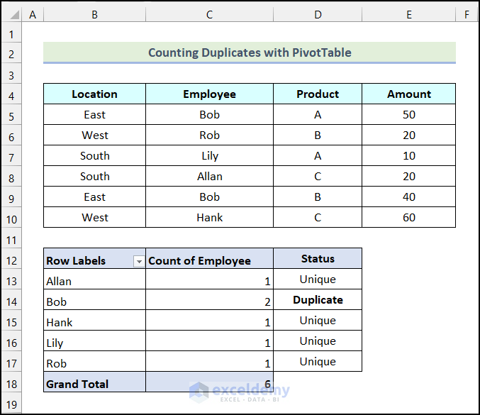
The following image demonstrates an overview of the steps discussed in this article.
How to Count Duplicates with Pivot Table in Excel: 3 Simple Steps
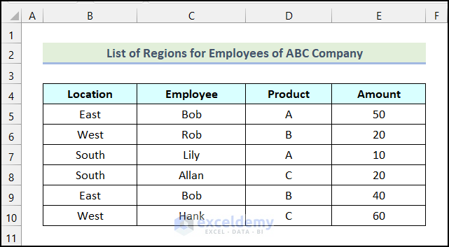
In this section of the article, we will learn three simple steps to count duplicates in Excel Pivot Table. Let’s say, we have the List of Regions for Employees of ABC Company as our dataset. Our goal is to count the duplicate values from the Employee column. Now, let’s use the steps mentioned in the following section to do this.
Step 01: Insert Pivot Table
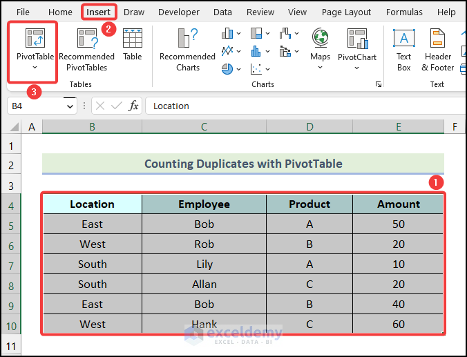
In the first step, we will insert the PivotTable using our dataset. So, let’s follow the instructions outlined below.
- Firstly, select the entire dataset and then go to the Insert tab from Ribbon.
- After that, click on the PivotTable option from the Tables group.
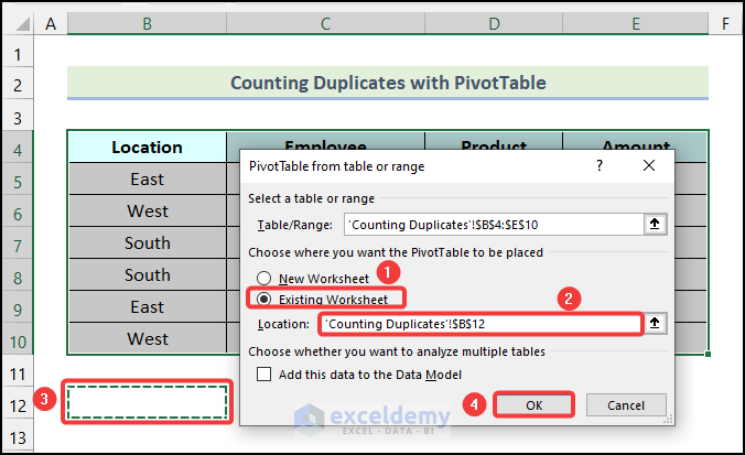
As a result, the PivotTable form table or range dialogue box will open on your worksheet.
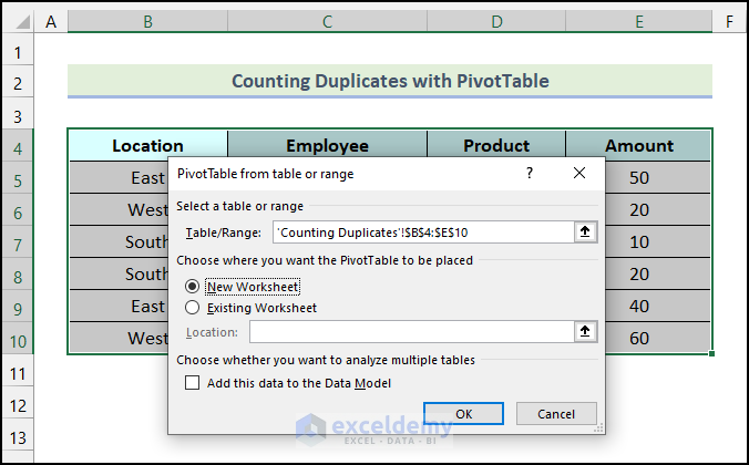
- Now, click on the Existing Worksheet option in the PivotTable form table or range dialogue box.
- Then, click on the Location field.
- Following that, select cell B12 as the destination cell of the PivotTable.
- Lastly, click on OK.
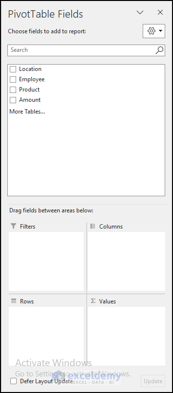
Consequently, the PivotTable Fields dialogue box will appear on your worksheet as shown in the following image.
Read More: How to Count Duplicate Values Only Once in Excel
Step 02: Define PivotTable Fields
In the second step, we will define the PivotTable Fields to count the duplicates. Now, let’s follow the steps given below.
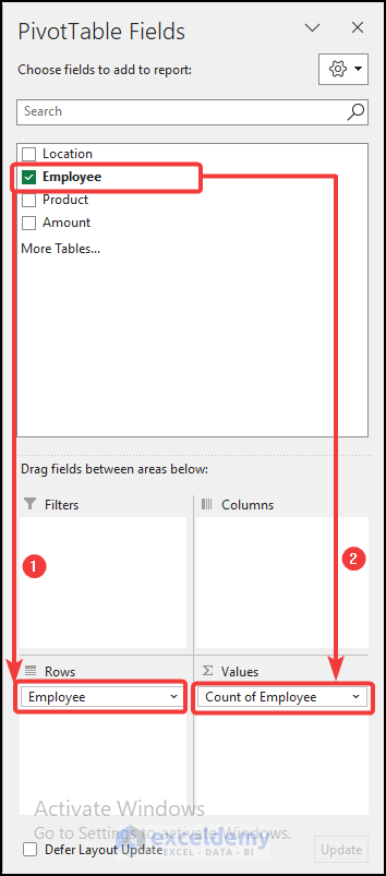
- Firstly, drag the Employee option to the Rows section in the PivotTable Fields dialogue box.
- Subsequently, again drag the Employee option to the Values section as demonstrated in the following picture.
Step 03: Find Count of Duplicates
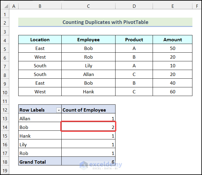
At this stage our Pivot Table is ready. Now, we need to identify the duplicates from the Pivot Table.
All the values that are 1 in the Count of Employee column are unique values. On the other hand, the values that are greater than 1 are our duplicate values.
- Now, identify any value that is greater than 1 in the Count of Employee column. In this case, Bob is the duplicate value.
How to Count Distinct Values in Excel Pivot Table
In this section of the article, we will discuss two different methods to count distinct values in Excel PivotTable. The distinct values are defined by such values that are present at least one time in a dataset. For example, if a value is repeated three times in a dataset, it will still be counted as one distinct value.
1. Using Helper Column
Inserting a helping column is the most available way to count distinct values in Excel pivot table. Here, we will use the same dataset that we used in the previous method. Now, let’s follow the step outlined in the following section.
Steps:
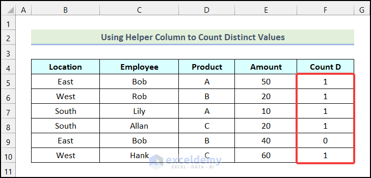
- Firstly, insert a helper column, ‘Count D’ in the F4:F10 range.
- Next, select cell F5 and type the following formula.
=IF(COUNTIFS($C$5:C5,C5,$B$5:B5,B5)>1,0,1)Formula Breakdown
- COUNTIFS($C$5:C5,C5,$B$5:B5,B5): Excel COUNTIFS function will return the number of cells from the given criteria range. Here this will return the number of C5 that exist between the criteria range1 $C$5:C5 & B5 from the criteria range2 $B$5:B5. We will need to make the first point of the range absolute to make it fixed. That means it won’t change by dragging.
- IF(COUNTIFS($C$5:C5,C5,$B$5:B5,B5)>1,0,1): Excel IF function will return 1 if the name is found for the first time and 0 if it is seen again.

- After that, press ENTER and use the Fill Handle tool to autofill the below cells.
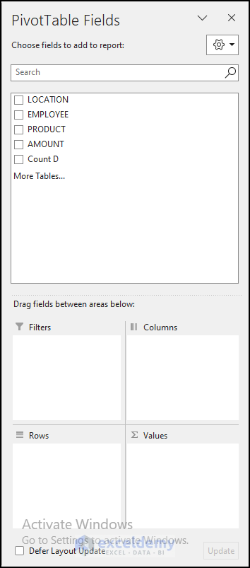
- Now, follow the steps mentioned in Step 01 of the first method and the PivotTable Fields dialogue box will open on your worksheet.
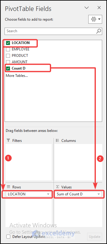
- Now, drag the Location option to the Rows section in the PivotTable Fields dialogue box.
- Following that, drag the Count D option to the Values section as shown in the following image.
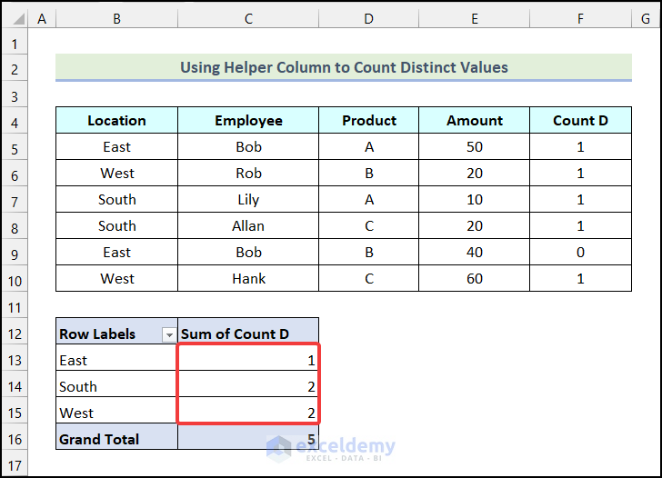
Consequently, the following PivotTable will appear on your worksheet. This indicates that the South and the West region have two distinct values. Whereas, the East region has only one distinct value although it has two entries.
Related Content: How to Ignore Blanks and Count Duplicates in Excel
2. Utilizing Data Model to Count Distinct Values
Utilizing the Data Model is another smart way to count distinct values in Excel PivotTable. Now, let’s follow the instructions discussed below to do this.
Steps:
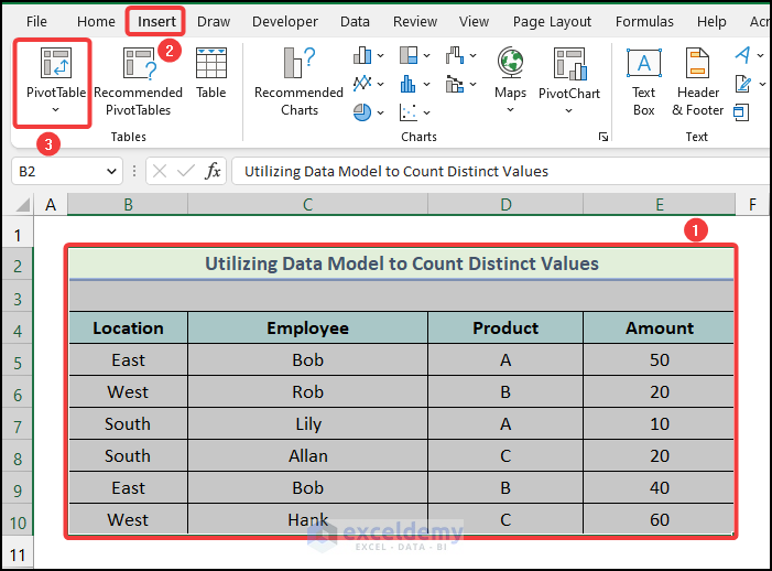
- Firstly, choose the entire dataset and then go to the Insert tab from Ribbon.
- Following that, click on the PivotTable option from the Tables group.
- Now, the PivotTable form table or range dialogue box will open on your worksheet. Then, click on the Existing Worksheet option there.
- Subsequently, click on the Location field.
- After that, select cell B12 as the destination cell of the PivotTable.
- Next, check the field named Add this data to Data Model.
- Finally, click on OK.

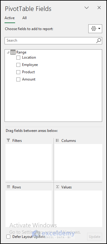
As a result, the PivotTable Fields dialogue box will open on your worksheet as demonstrated in the image below.
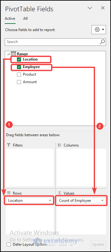
- Now, drag the Location option to the Rows section in the PivotTable Fields dialogue box.
- After that, drag the Employee option to the Values section as shown in the following picture.
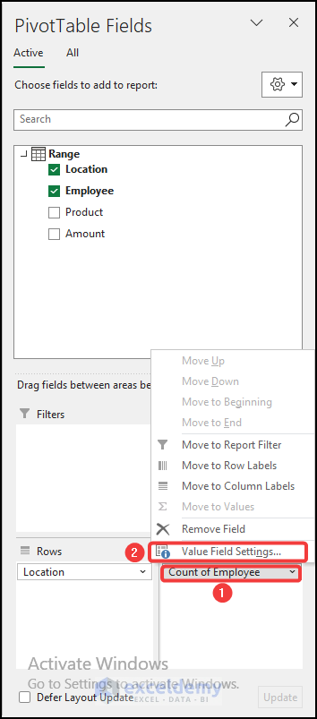
- Subsequently, click on the Count of Employee option as marked in the picture below.
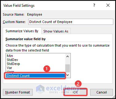
- Then, choose the Value Field Settings from the available options.
As a result, the Value Filed Settings dialogue box will be available on your worksheet.
- Now, select the Distinct Count option in the Value Field Settings dialogue box.
- Finally, click OK.
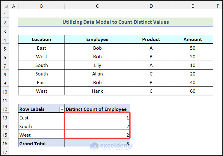
Consequently, the distinct values from the dataset will be available in the PivotTable shown in the following image.
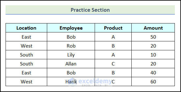
Practice Section
In the Excel Workbook, we have provided a Practice Section on the right side of the worksheet. Please practice it yourself.
Read More: How to Use COUNTIF Formula to Find Duplicates
Download Practice Workbook
Conclusion
So, these are the most common and effective methods you can use anytime while working with your Excel datasheet to count duplicates in Excel Pivot Table. If you have any questions, suggestions, or feedback related to this article, you can comment below.
Related Articles
- How to Count Repeated Words in Excel
- VBA to Count Duplicates in Range in Excel
- Excel VBA to Count Duplicates in a Column
<< Go Back to Count Duplicates in Excel | Duplicates in Excel | Learn Excel
Get FREE Advanced Excel Exercises with Solutions!
