An Example of the COUNTIF Formula:
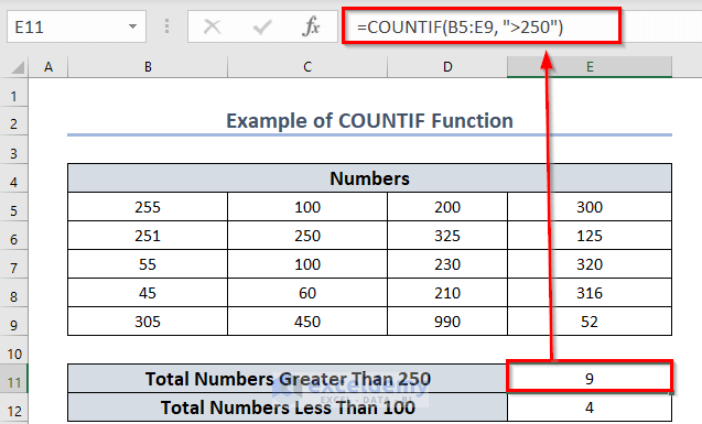
COUNTIF(B5:E9, “>250”): Count the value if it is greater than 250 in the cell range B5 to E9.
Now, observe the following image. Here, I have applied the following formula in cell E11.
=COUNTIF(B5:E9, ">250")Here, E11 displays the total numbers that are greater than 250 in the cell range B5 to E9.
How to Use the COUNTIF Formula to Find Duplicates: 5 Easy Ways
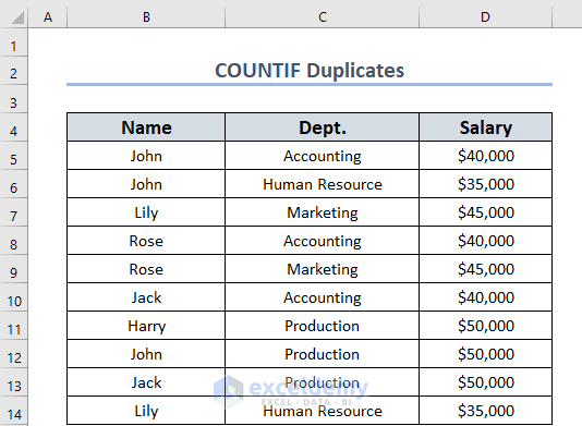
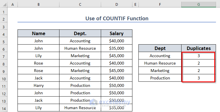
We’ll use the following dataset which has 3 columns: Name, Dept., and Salary. We’ll find the duplicated values across the columns.
Method 1 – Using the COUNTIF Function to Find Duplicates in a Range Counting First Occurrence
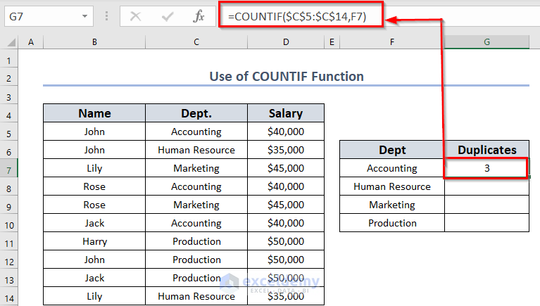
- Make a smaller table to the side to put values that you want to search for (see screenshot below).
- Click on the G7 cell to select it.
- Use this formula in this cell:
=COUNTIF($C$5:$C$14,F7)The formula counts the number of values equal to the value in F7 in the data range $C$5:$C$14.
- Press Enter to get the result.
- Go to the bottom-right corner of cell G7, and the icon will change to a plus called the Fill Handle icon. Click the Fill Handle icon, hold it, and drag until you reach cell G10.
- Release the mouse button.
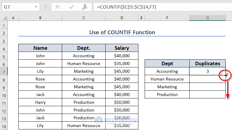
- You will get the following result.
Read More: How to Ignore Blanks and Count Duplicates in Excel
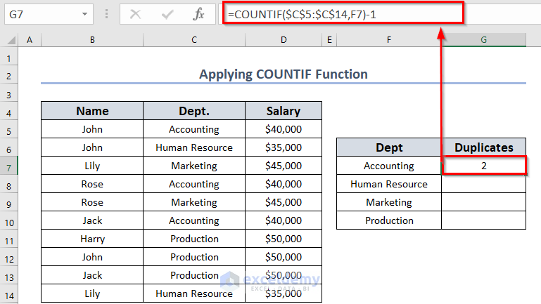
Method 2 – Counting Duplicate Values without the First Occurrence
- Click the G7 cell to select it.
- Use this formula:
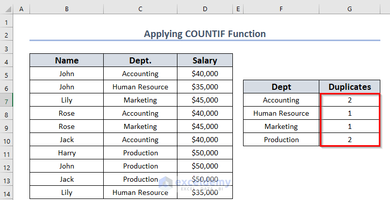
=COUNTIF($C$5:$C$14,F7)-1This is effectively the same formula as before but subtracts 1. If the value isn’t found, it’ll yield -1.
- Press Enter to get the result.
- Drag the Fill Handle icon to AutoFill the corresponding data in the rest of the cells G8:G10.
Read More: How to Count Duplicate Values Only Once in Excel
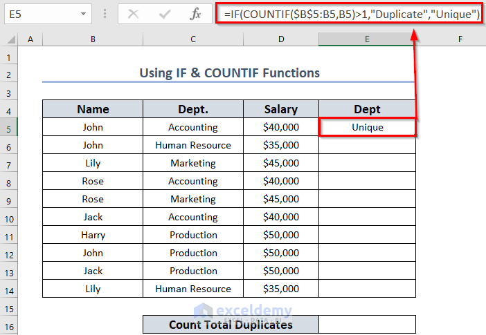
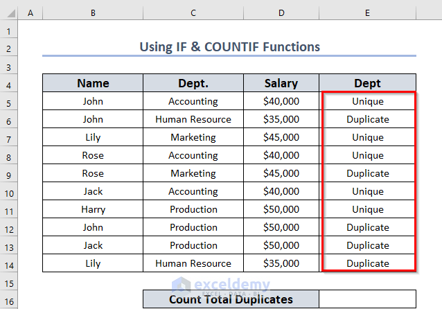
Method 3 – Use COUNTIF and IF Functions to Find Duplicates in a Column
- Make a new column E to display the results.
- Click the E5 cell to select it.
- Use this formula:
=IF(COUNTIF($B$5:B5,B5)>1,"Duplicate","Unique")- Press Enter to get the result.
Formula Breakdown
- The COUNTIF function will count those cells whose values fulfill the criteria.
- For the first cell, COUNTIF($B$5:B5,B5) becomes 1.
- Here, the IF function will check the given logical test.
- COUNTIF($B$5:B5,B5)>1 denotes the logical test. This test will check whether the count number is greater than 1.
- When the number is greater than 1 then it will return Duplicate.
- If the logic test fails the formula will return Unique.
- So, IF(1>1,”Duplicate”,”Unique”) returns Unique.
- Drag the Fill Handle icon to AutoFill the corresponding data in the rest of the cells E6:E14.
- Enter the formula given below in the E16 cell to find the total duplicates.
=COUNTIF(E5:E14,"Duplicate")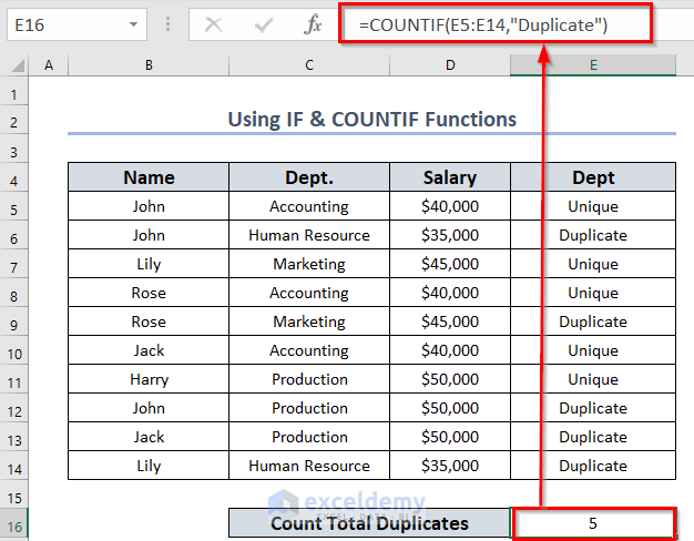
Read More: How to Count Repeated Words in Excel
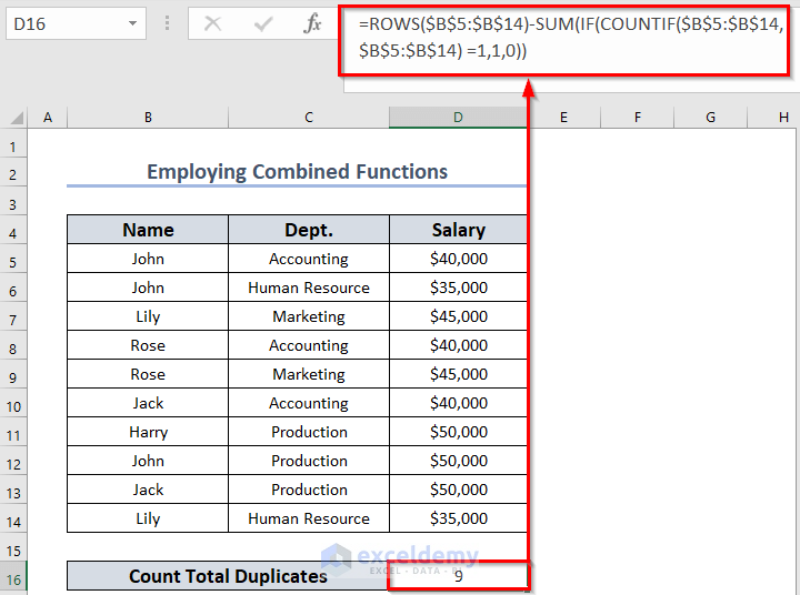
Method 4 – Finding Total Duplicates in a Column Including First Occurrence
Steps:
- Select a new cell D16, where you want to keep the result.
- Use the following formula:
=ROWS($B$5:$B$14)-SUM(IF(COUNTIF($B$5:$B$14,$B$5:$B$14) =1,1,0))- Press Enter.
Formula Breakdown
- COUNTIF($B$5:$B$14,$B$5:$B$14)—> becomes {3,3,2,2,2,2,1,3,2,2}
- IF(COUNTIF($B$5:$B$14,$B$5:$B$14) =1,1,0)—> turns {0,0,0,0,0,0,1,0,0,0}
- SUM(0,0,0,0,0,0,1,0,0,0)—> gives 1.
- ROWS($B$5:$B$14)—> returns 10.
- Output: 10-1 = 9.
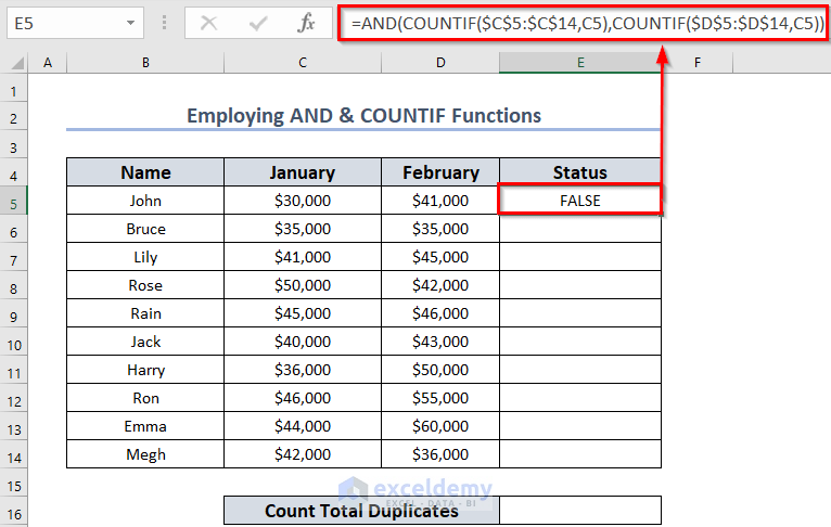
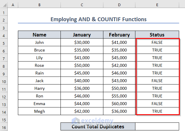
Method 5 – Applying AND and COUNTIF Functions to Find Duplicate Values within Multiple Columns
We’ll count the duplicates between the January and February columns.
- Select a new cell, E5, where you want to keep the result.
- Use the formula given below:
=AND(COUNTIF($C$5:$C$14,C5),COUNTIF($D$5:$D$14,C5))- Press Enter to get the result.
Formula Breakdown
- Here, $C$5:$C$14 is the range of the January column and $D$5:$D$14 is the range of the February column.
- COUNTIF($C$5:$C$14,C5)—> returns the number of the value in cell C5 in the range $C$5:$C$14.
- Output —> 1
- COUNTIF($D$5:$D$14,C5) —> returns the number of the value in cell C5 in the range $D$5:$D$14
- Output—> 0
- AND(COUNTIF($C$5:$C$14,C5),COUNTIF($D$5:$D$14,C5)) —> becomes AND(1,0)
- Output—> FALSE
- Drag the Fill Handle icon to AutoFill the corresponding data in the rest of the cells E6:E14.
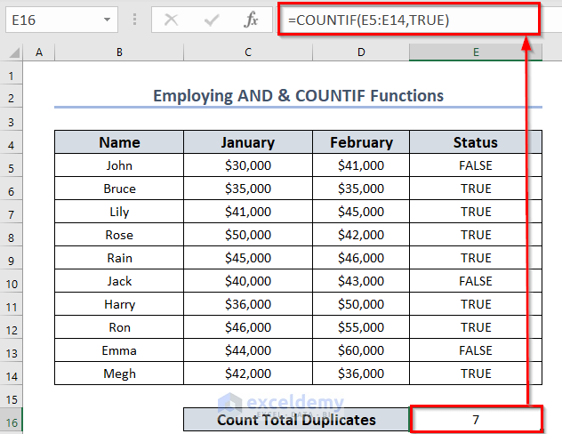
- Use the formula given below in the E16 cell to find the total duplicates.
=COUNTIF(E5:E14,TRUE)- Press Enter to get the result. You will get the total duplicate number.
Read More: VBA to Count Duplicates in Range in Excel
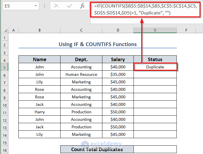
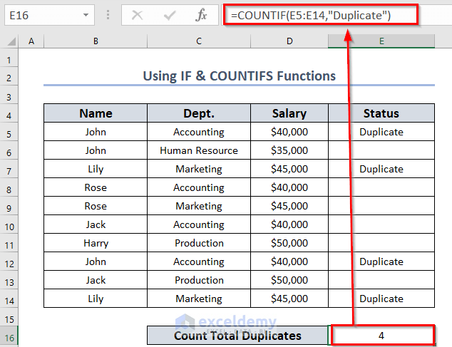
Use the COUNTIFS Function to Find Duplicate Rows in Excel
Steps:
- Select cell E5 and insert the following formula:
=IF(COUNTIFS($B$5:$B$14,$B5,$C$5:$C$14,$C5,$D$5:$D$14,$D5)>1, "Duplicate", "")- Press Enter.
Formula Breakdown
- $B$5:$B$14 is the data range 1 and $B5 is the criteria 1.
- $C$5:$C$14 is the data range 2 and $C5 is the criteria 2.
- $D$5:$D$14 is the data range 3 and $D5 is the criteria 3.
- COUNTIFS($B$5:$B$14,$B5,$C$5:$C$14,$C5,$D$5:$D$14,$D5)—> becomes 2.
- IF(2>1, “Duplicate”, “”)—> gives Duplicate.
- Double-click on the Fill Handle icon to AutoFill the corresponding data in the rest of the cells E6:E14.
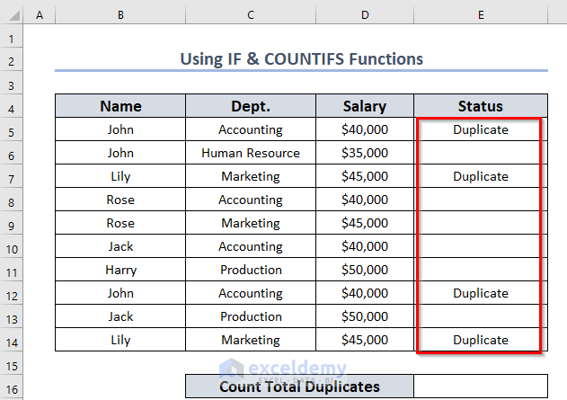
- Use the formula given below in the E16 cell to find the total number of duplicates.
=COUNTIF(E5:E14,"Duplicate")- Press Enter to get the result.
Read More: Excel VBA to Count Duplicates in a Column
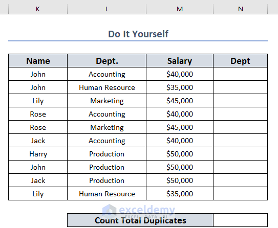
Practice Section
You can practice the explained methods in the download document.
Download the Practice Worksheet
<< Go Back to Count Duplicates in Excel | Learn Excel
Get FREE Advanced Excel Exercises with Solutions!
