Reverse Legend Order of Stacked Bar Chart in Excel (With Quick Steps)

In this article, we will learn to reverse the legend order of a stacked bar chart in Excel. A stacked bar chart is a graph that uses bars to show different data. Generally, it is used to break down and compare different parts of a whole. Today, we will demonstrate step-by-step procedures to reverse the legend order of the stacked bar chart in Excel. So, without any delay, let’s start the discussion.

Download Practice Book

You can download the practice book from here.

Step-by-Step Procedures to Reverse Legend Order of Stacked Bar Chart in Excel

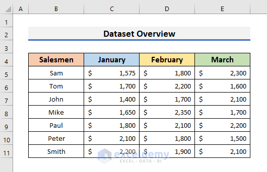
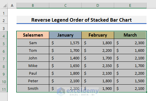
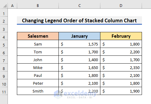
To explain the steps, we will use a dataset that contains the sales amount of some Salesmen for January, February, and March. We will create a stacked bar chart using these values and then, try to reverse the legend order.

STEP 1: Create Stacked Bar in Excel

• In the first place, create a stacked bar in Excel.
• To do so, select all the cells of the dataset.

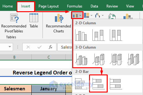
• After that, go to the Insert tab and select the Insert Column or Bar Chart icon. A drop-down menu will appear.
• Select 2-D Stacked Bar from there.

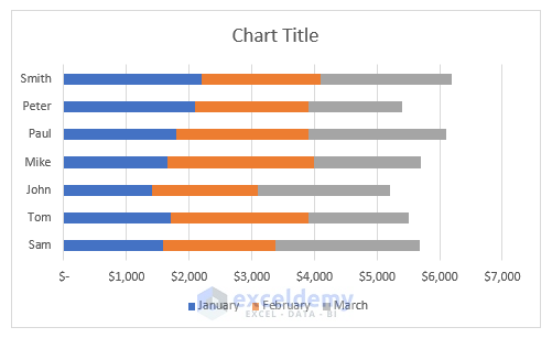
• Instantly, a 2-D Stacked Bar will appear on the excel sheet.

Read More: How to Create Stacked Bar Chart with Line in Excel (2 Suitable Examples)

STEP 2: Open Context Menu and Select Data

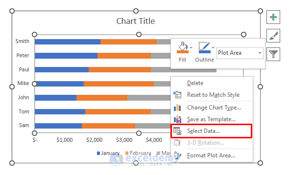
• Secondly, right–click on the chart to open the Context Menu.
• In the Context Menu, click on the Select Data option.
• It will open the Select Data Source window.

Read More: How to Change Bar Chart Width Based on Data in Excel (with Easy Steps)

Similar Readings

• How to Make a Simple Bar Graph in Excel (with Easy Steps)
• How to Make a Double Bar Graph in Excel (with Easy Steps)
• Excel Stacked Bar Chart with Subcategories (2 Examples)
• How to Change Bar Chart Color Based on Category in Excel (3 Methods)
• What is the Difference Between Bar Graph and Histogram?

STEP 3: Reverse Position of Legend Entries

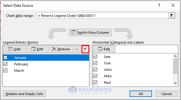
• Thirdly, you need to reverse the position of the legend entries.
• In our case, the order of the legends is January, February, and March.

• In order to reverse the order, select January and click on the drop–down arrow twice in the Legend Entries section.

• Again, select February and click on the drop–down arrow once.

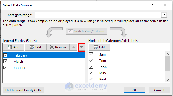
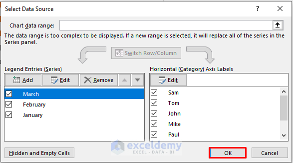
• After that, the order in the Legend Entries will be March, February, and January.
• Press OK.

Final Output

• Finally, after clicking OK, you will see the reverse legend order of the stacked bar chart.

Change Legend Order of Stacked Column Chart in Excel

In this section, we will learn to change the legend order of the stacked column chart in Excel. We will use the manual method here. To explain this process, we will use the previous dataset but we will consider the first two months only.

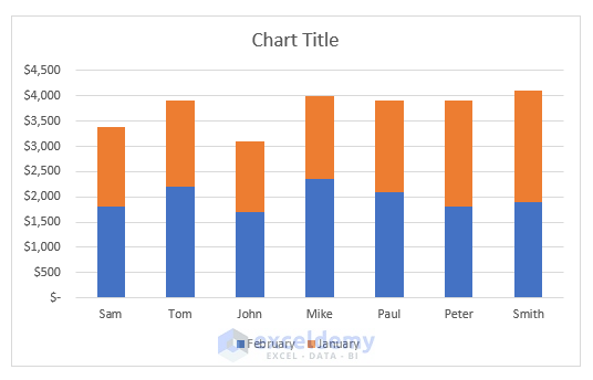
The stacked column chart of the above dataset looks like the graph below.

Let’s observe the steps below to learn more about the method.

STEPS:

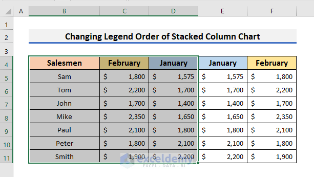
• Firstly, create duplicate columns of February and January with zeros in Columns C and D respectively.
• Remember, the duplicate columns should be in reverse order.

• Secondly, fill in the sales amount for February and January.

• After that, select the range B4:D11.

• In the following step, navigate to the Insert tab and select the Insert Column or Bar Chart icon. A drop-down menu will appear.
• Select the Stacked Column icon from there.

• Finally, you will see the change in legend order of the stacked column chart in Excel.

Read More: How to Make a 100 Percent Stacked Bar Chart in Excel (with Easy Steps)

Conclusion

In this article, we have demonstrated step-by-step procedures to Reverse Legend Order of Stacked Bar Chart in Excel. I hope this article will help you to perform your tasks easily. Moreover, we have also added the practice book at the beginning of the article. Furthermore, you can download it to test your skills. Visit the ExcelDemy website for more articles like this. Last of all, if you have any suggestions or queries, feel free to ask in the comment section below.

Related Articles

• How to Make a Bar Graph in Excel with 2 Variables (3 Easy Ways)
• How to Add Vertical Line to Excel Bar Chart (3 Quick Ways)
• Excel Add Line to Bar Chart (4 Ideal Examples)
• How to Show Percentage in Bar Chart in Excel (3 Handy Methods)
• How to Plot Stacked Bar Chart from Excel Pivot Table (2 Examples)
• Excel Chart Bar Width Too Thin (2 Quick Solutions)