How to Add the Grand Total to a Bar Chart in Excel – Easy Steps

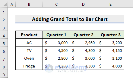
The sample dataset showcases 4 different products and their sales in 3 quarters.

STEP 1 – Insert a Spacing and a Grand Total Column

• Insert 2 extra columns.
• In the first column (Spacing), enter 10,000 for every product.

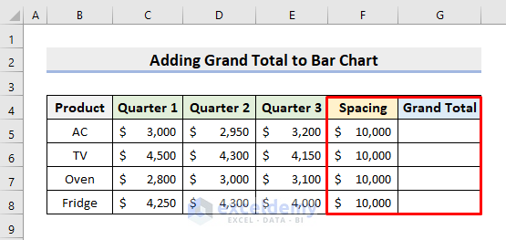
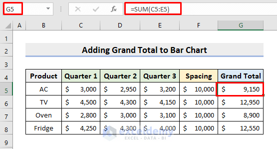
In the Grand Total column, add the sales to find the total:

• Select G5.
• Enter the formula:

• Press Enter.
• Use AutoFill to see the sales summation of other products.

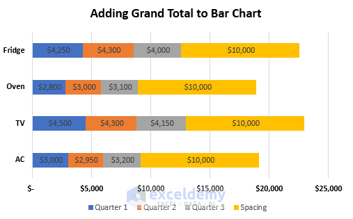
STEP 2 – Insert a Bar Chart in Excel

• Select B4:F8.

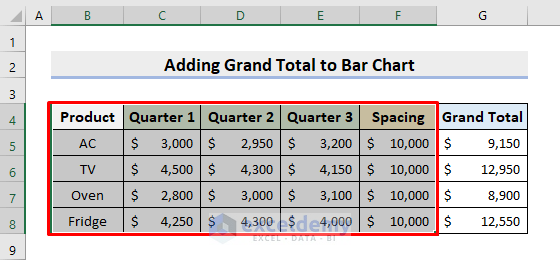
• Go to Insert ➤ Insert Column or Bar Chart ➤ 2-D Stacked Bar Chart.

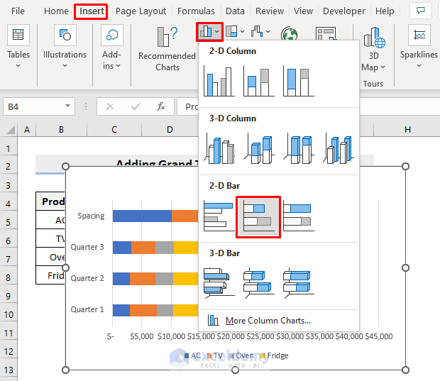
• The bar chart will be displayed.
• Click the chart.
• Select Chart Design ➤ Switch Row/Column.

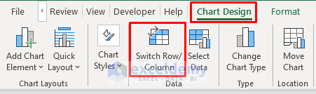
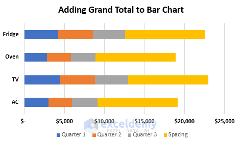
This is the output.

Read More: How to Change Bar Chart Color Based on Category in Excel

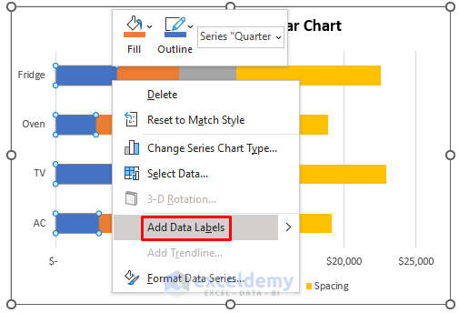
STEP 3 – Modify the Bar Chart to Add the Grand Total

• Right-click Quarter 1.
• Select Add Data Labels.
• Repeat the steps for the other parts of the chart.

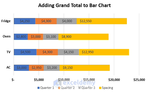
Data labels will be displayed.

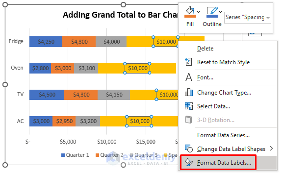
• Right-click Spacing (10,000).
• Select Format Data Labels.

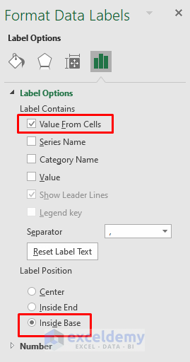
• In the Format Data Labels pane, choose Inside Base in Label Position.
• Check Value From Cells in Label Options.

• In the dialog box, choose the Grand Total range in Select Data Label Range.

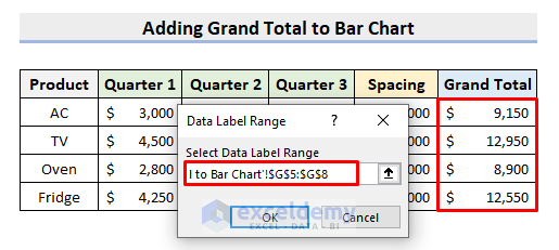
• Click OK.

This is the output.

• Right-click Spacing.
• Choose No Fill in Fill.

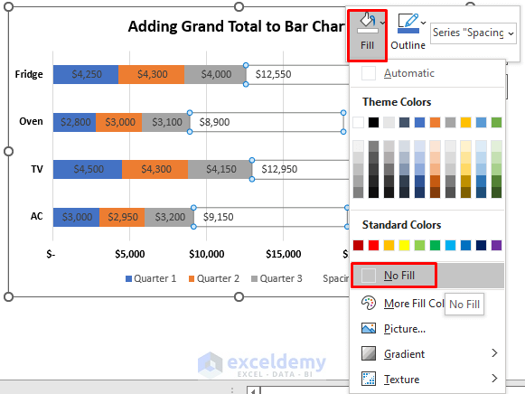
• Delete the y-axis lines.
• Delete the Spacing legend.

Read More: How to Color Bar Chart by Category in Excel

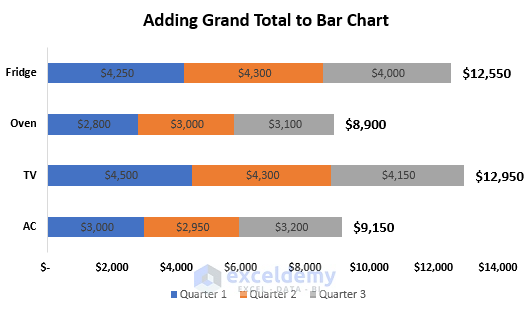
STEP 4 – Change Spacing Column Values

• Enter 0 for every product in the Spacing column.

Read More: Excel Add Line to Bar Chart

Final Output

• Choose a format for the Grand Total data labels.

This is the final output.

Download Practice Workbook

Download the workbook to practice.

Related Articles

• How to Create Bar Chart with Error Bars in Excel
• How to Sort Bar Chart in Descending Order in Excel
• Excel Bar Graph Color with Conditional Formatting
• How to Add Horizontal Line to Bar Chart in Excel
• How to Add Vertical Line to Excel Bar Chart
• How to Create Bar Chart with Target Line in Excel
• Excel Bar Chart with Line Overlay

<< Go Back to Excel Bar Chart | Excel Charts | Learn Excel