How to Sort Bar Chart in Descending Order in Excel (4 Easy Ways)

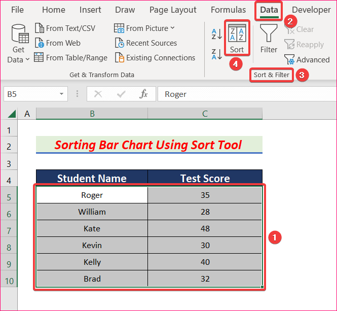
We will use the following dataset, which contains two columns named Student Name and Test Score. A bar chart is inserted using these two columns.

Method 1 – Sort a Bar Chart Using the Sort Tool

We’ll sort the chart in ascending order by test scores.

Steps:

• Select all the data from both columns.
• Go to Data, then to Sort & Filter, and select Sort.

• The Sort dialogue box will appear.
• Check the box for My data has headers.
• Choose Test Score in the Sort by option.
• Choose the Smallest to Largest in Order option.

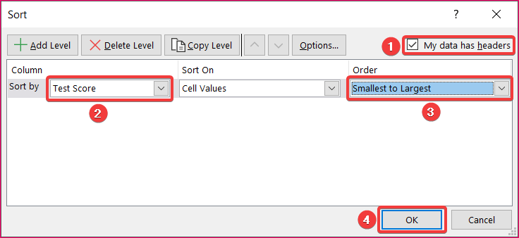
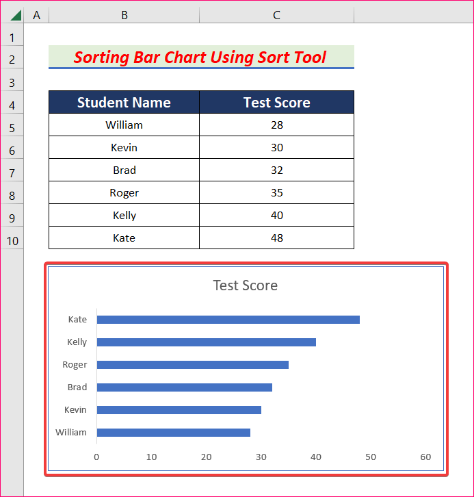
• Click OK and you will find your bar chart sorted in descending order.

Read More: How to Sort Bar Chart Without Sorting Data in Excel

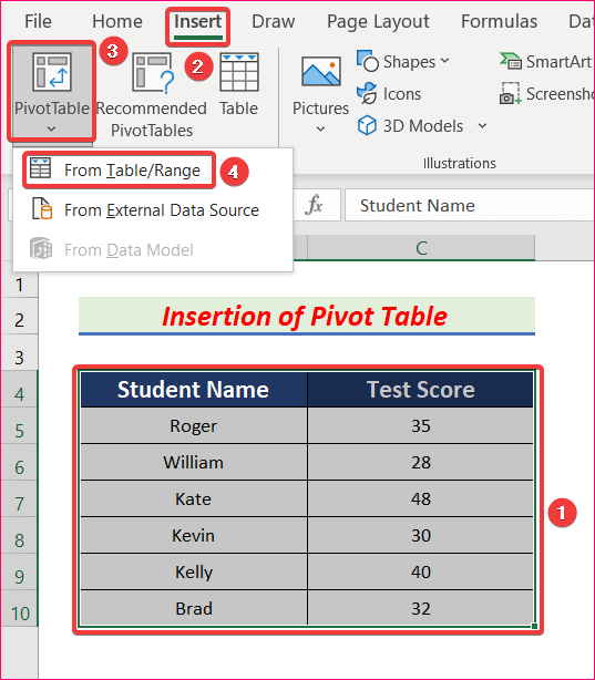
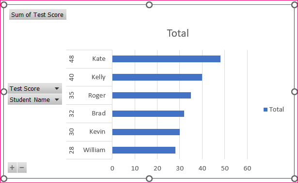
Method 2 – Insert a Pivot Table to Sort a Bar Chart in Reverse Order

Steps:

• Select both Student Name and Test Score columns.
• From the Insert tab, go to PivotTable and select From Table/Range.

• A new dialog box will pop up.
• Select Existing Worksheet and choose a Location.

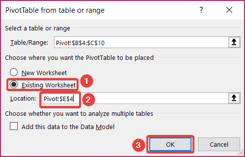
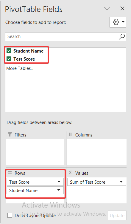
• Once you click OK, the Pivot Table Fields panel will open.
• Check both the Student Name and Test Score from there and drag them under the Rows field.

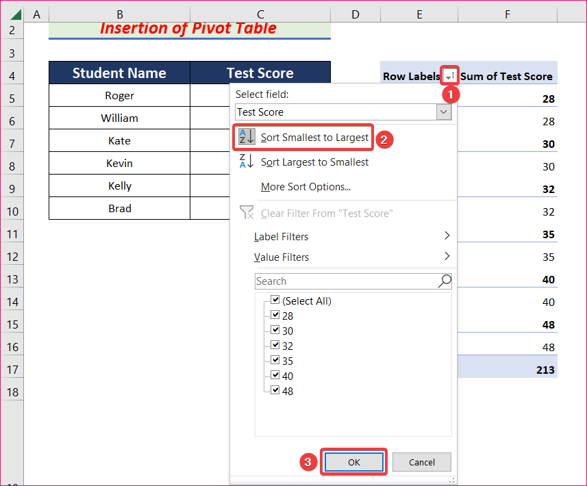
• Go to the pivot table and click on the dropdown beside Row Labels.
• Select Sort Smallest to Largest and click OK.

• Click on the Insert tab and go to Charts, then to Insert Column or Bar Chart, and pick Clustered Bar.

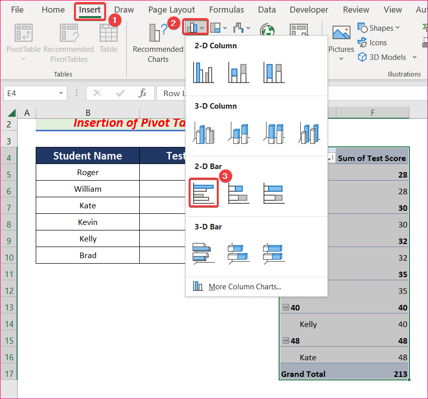
• You will get your bar chart arranged in descending order.

Read More: How to Change Bar Chart Color Based on Category in Excel

Method 3 – Use Categories in the Reverse Order Option

This method only works if the data in the table is sorted from largest to smallest.

Steps:

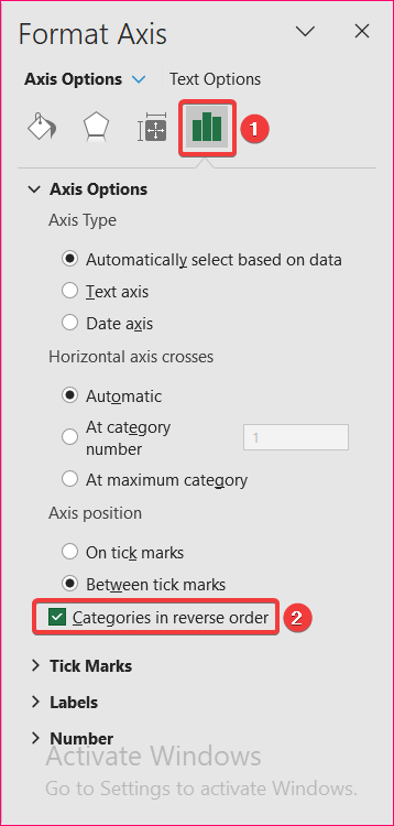
• Right-click on the vertical axis of the bar chart and select Format Axis.

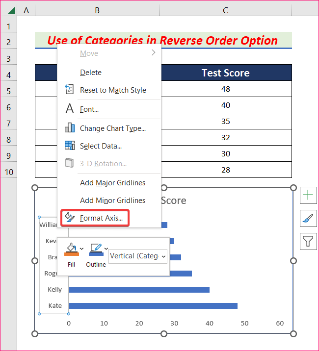
• From Axis Options, check the box for Categories in reverse order.

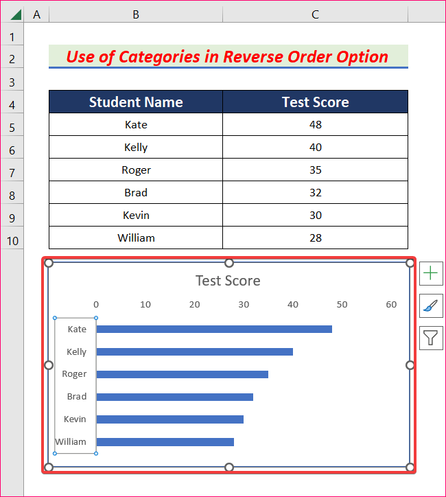
• You will see that the bar chart is arranged in descending order.

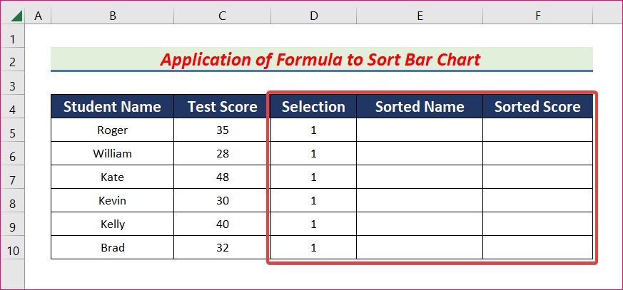
Method 4 – Apply a Formula to Sort the Bar Chart in Descending Order

Steps:

• Add three new columns named Selection, Sorted Name, and Sorted Score.
• Fill the Selection column with the value 1.

• Select cell E5, insert the following formula, and press Enter.

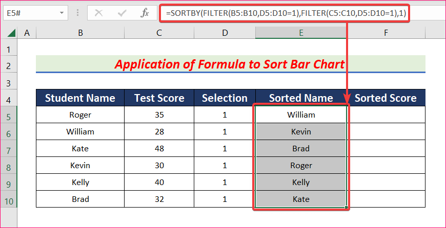
• Select cell F5 and apply the formula given below.

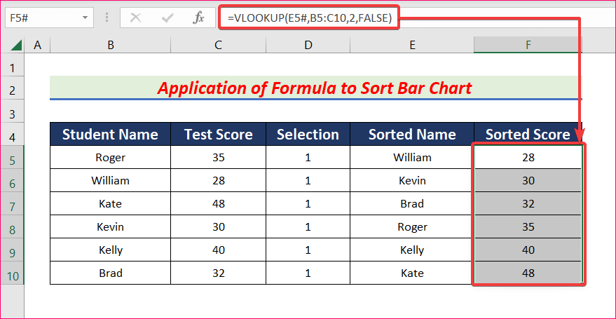
• Click on the Insert tab, go to Insert Column or Bar Chart and pick a Clustered Bar.

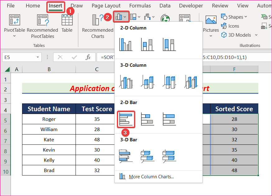
• You will get your bar chart in descending order.

Read More: How to Add Grand Total to Bar Chart in Excel

Download the Practice Workbook

Related Articles

• How to Create Bar Chart with Error Bars in Excel
• How to Color Bar Chart by Category in Excel
• Excel Bar Graph Color with Conditional Formatting
• Excel Add Line to Bar Chart
• How to Add Horizontal Line to Bar Chart in Excel
• How to Add Vertical Line to Excel Bar Chart
• How to Create Bar Chart with Target Line in Excel
• Excel Bar Chart with Line Overlay

<< Go Back to Excel Bar Chart | Excel Charts | Learn Excel