In this article, we will walk through 4 easy and effective methods to create an Excel Bar Chart that ignores blank cells.
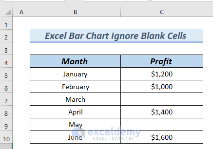
To illustrate our methods, we’ll use the following dataset containing Month and Profit columns. In the Profit column the values for the months of March and May are blank in cells C7 and C9. We’ll insert a Bar chart using this data table that ignores the blank cells.
We used Excel 365 to perform all operations in this article.
Method 1 – Using 2D Bar Chart to Ignore Blank Cells
In this method, we will insert a 2D Bar chart using our dataset, then use the Select Data feature to select Zero (0) to Show empty cells.
Step 1 – Inserting 2D Bar Chart
First we insert the Bar chart.
- Select the entire dataset.
- Go to the Insert tab.
- From Insert Column or Bar Chart group, select 2D Clustered Bar chart.
![]()
The Bar chart is inserted.
- Click on the Chart Title to edit it.
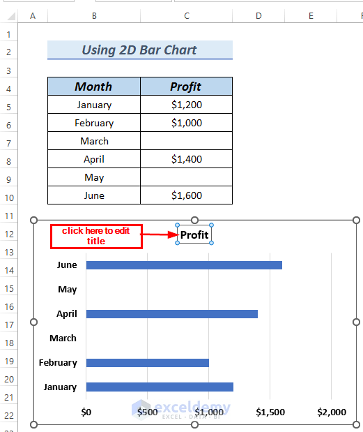
The Bar chart has an edited Chart Title.
![]()
Step 2 – Adding Data Label to Bar Chart
Now we add Data Labels to our Bar chart.
- Click on the chart and select Chart Elements.
- Mark Data Labels.
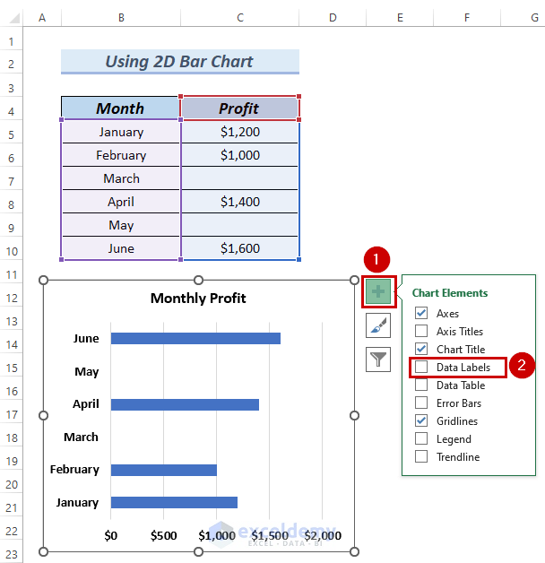
Data Labels are added to the chart.
As the months of March and May have blank cells, the chart has no data labels for these two months, so it looks incomplete.
![]()
Step 3 – Using Select Data Feature to Ignore Blank Cells
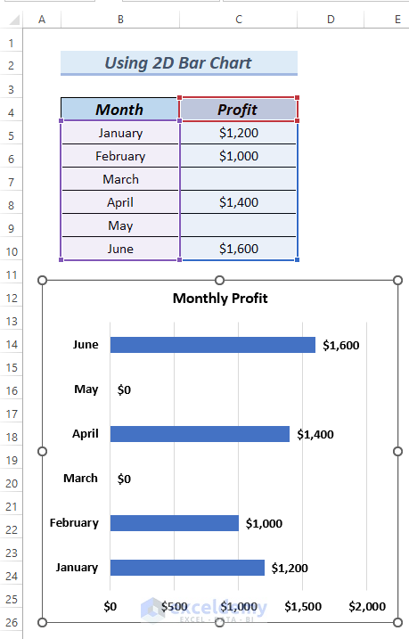
Now we use the Select Data feature to select Zero (0) to Show empty cells. The blank months in the chart will then have 0 as a value.
- Right-click on the chart.
- Select Select Data from the Context Menu.
![]()
A Select Data Source dialog box will appear.
- Click on Hidden and Empty Cells.
![]()
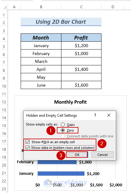
A Hidden and Empty Cell Settings dialog box will appear.
- Select Show empty cells as Zero.
- Mark both the Show #N/A as an empty cell box and the Show data in the hidden rows and columns boxes.
- Click OK.
- Click OK in the Select Data Source dialog box.
![]()
The months of March and May is showing $0 instead of blanks.
Read More: How to Make a Stacked Bar Chart in Excel
Method 2 – Inserting 3D Bar Chart to Ignore Blank Cells
This method is similar to the first, but we will insert a 3D Bar chart using our dataset.
Steps:
First, we will insert a 3D Bar chart.
- Select the entire dataset.
- Go to the Insert tab.
- Select Recommended Charts.
![]()
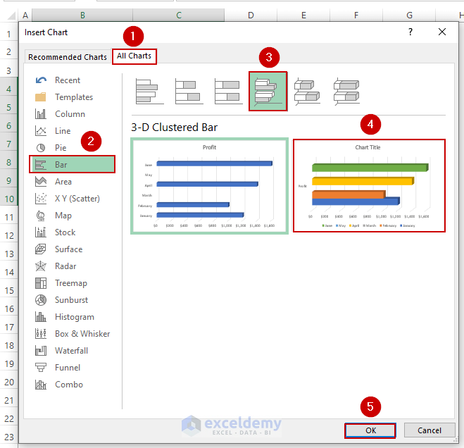
An Insert Chart dialog box will appear.
- Go to All Charts >> select Bar.
- From 3D Clustered Bar Group, select the colored Bar Chart.
- Click OK.
The 3D Bar chart is inserted.
- Click on the Chart Title to edit the Chart Title.
![]()
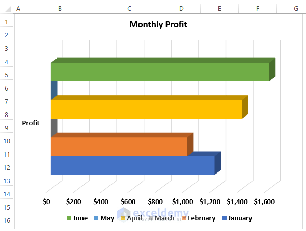
The 3D Bar chart has an edited Chart Title.
- Follow Step 2 of Method 1 to add Data Labels to the 3D Bar chart.
- Follow Step 3 of Method 1 to go through the Select Data feature to select Zero (0) as Show empty cells.
The months of March and May now show $0 instead of blanks.
![]()
Read More: How to Create Stacked Bar Chart with Negative Values in Excel
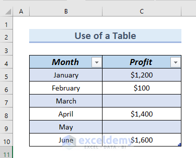
Method 3 – Using a Table to Ignore Blank Cells in Excel Bar Chart
In this method, we will insert a Table in our dataset, filter the blank cells out of the table, then insert a Bar chart.
Step 1 – Inserting Table
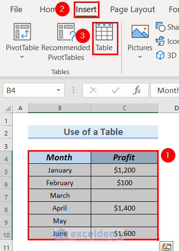
First we insert a Table using our dataset.
- Select the entire dataset. You can select cell B4 and use the keyboard shortcut CTRL+SHIFT+END to select the entire dataset quickly.
- Go to the Insert tab.
- From the Tables group, click on Table.
A Create Table dialog box will appear.
- Make sure My table has headers is marked.
- Click OK.
![]()
The Table is created.
- Change the Table header’s text color to Black to make them more visible.
Step 2 – Filtering Data Table
Next we will Filter out the Blank cells from the table.
- Click on the drop-down arrow of the Profit column.
![]()
A dialog box appears.
In the Number Filters group, all the numerical values are selected including the Blanks.
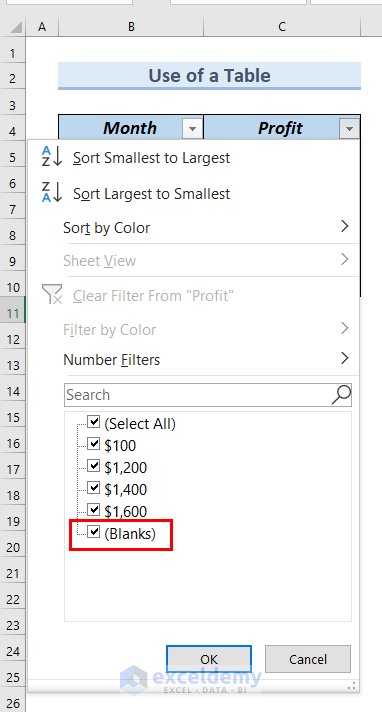
- Unmark the Blanks.
![]()
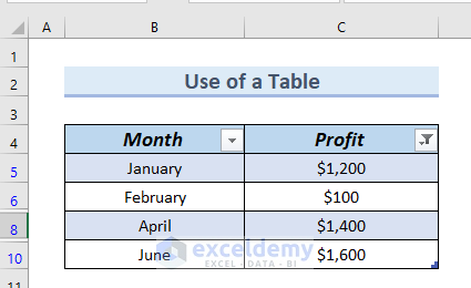
The table now contains no blank cells.
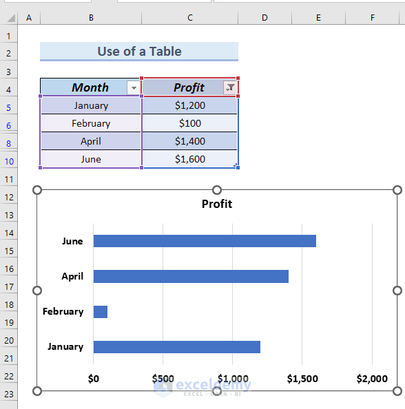
Step 3 – Inserting Bar Chart
Next we insert a Bar chart using the Table.
- Select the entire Table.
- Go to the Insert tab.
- From Insert Column or Bar Chart, select a Clustered Bar Chart.
![]()
The Excel Bar chart now ignores the blank cells.
Read More: How to Create Stacked Bar Chart for Multiple Series in Excel
Method 4 – Using Combined Functions to Ignore Blank Cells
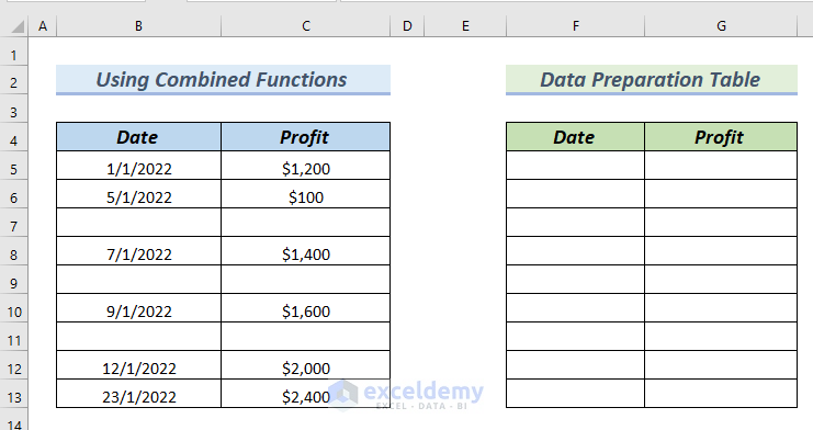
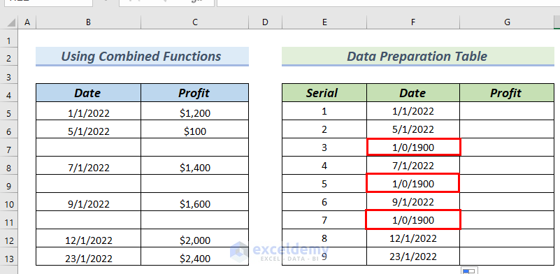
The following dataset contains Date and Profit columns. There are a number of blank cells in both the Date and the Profit columns. We will use the combination of the INDEX, AGGREGATE, IFERROR, ROW, and ROWS functions to remove the blank cells from the Date column. We will also use the combination of the INDEX and MATCH functions to remove the blank cells of the Profit column. Then we will insert a Bar chart. As a result, we will have an Excel Bar chart that ignores blank cells.
![]()
Step 1 – Finding Date in Data Preparation Table by Using Index Function
First we will use the INDEX function to find the date in the Data Preparation Table.
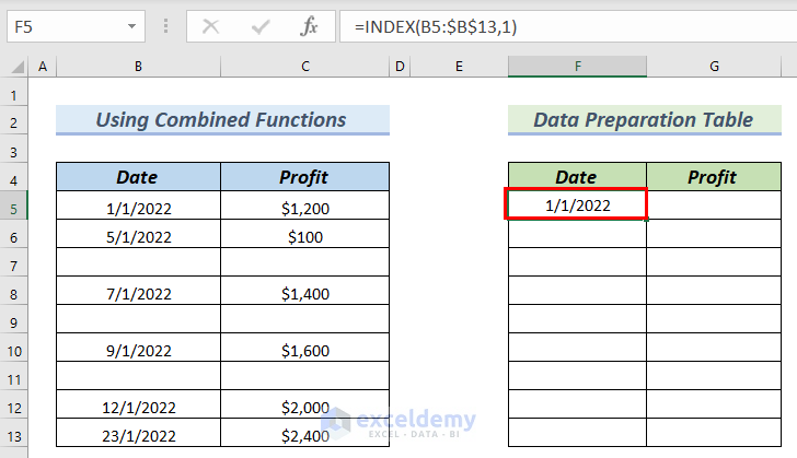
- Enter the following formula in cell F5:
=INDEX($B$5:$B$13,1)![]()
Formula Breakdown
- INDEX($B$5:$B$13,1) the INDEX function → the INDEX function returns the value of an item in an array or table that is chosen by the indexes of a column and row number.
- $B$5:$B$13 → is the array.
- 1 → is the specified row number.
- INDEX($B$5:$B$13,1) → becomes
- Output: 44562
- Explanation: 44562 is the Date in cell F5.
- Press ENTER to display the result in cell F5.
A number is shown in cell F5 instead of a Date. We have to format cell F5 with Date format to display it as a Date.
- Select cell F5 and go to the Home tab.
- Click on the downward arrow of the Number Format box.
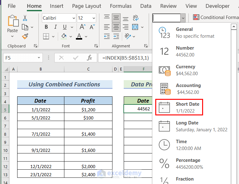
- Select Short Date.
![]()
In cell F5, the date is showing.
Step 2 – Adding Serial to Date Column
Now we will add a Serial column to our Data Preparation Table. The Serial column indicates a serial from 1 to 9. The previous formula in cell F5 was:
=INDEX($B$5:$B$13,1)
We will replace 1 with E5, so the formula becomes:
=INDEX($B$5:$B$13,E5)![]()
Formula Breakdown
- INDEX($B$5:$B$13,E5): The INDEX function → returns the value of an item in an array or table that is chosen by the indexes of the column and row number.
- $B$5:$B$13 is the array.
- E5 is the specified row number.
- INDEX($B$5:$B$13,E5) becomes
- Output: 1/1/2022
- Explanation: 44562 is the Date in cell F5.
- Press ENTER to return the result in cell F5.
- Drag down the formula with the Fill Handle tool.
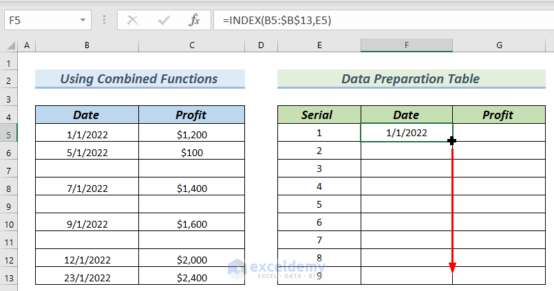
Cells F7, F9, and F11 have date values that are not real dates, because the cells B7, B9, and B11 have blank cells.
Step 3 – Adding Row Number by Using AGGREGATE and ROW Functions
Next, we will add a Row Number to our Data Preparation Table, using the combination of AGGREGATE and ROW functions.
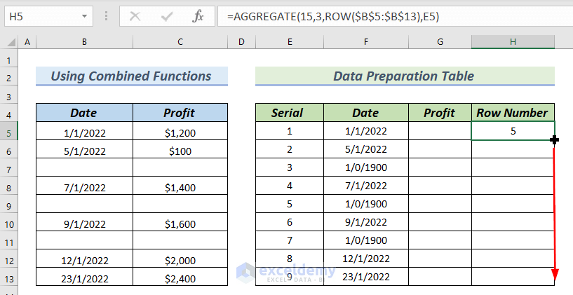
- Enter the following formula in cell H5:
=AGGREGATE(15,3,ROW($B$5:$B$13),E5)![]()
Formula Breakdown
- AGGREGATE(15,3,ROW($B$5:$B$13),E5) → the AGGREGATE function has multiple options for avoiding hidden rows along with error values.
- 15 → is the SMALL function_num.
- 3 → is the options that ignore hidden rows, error values, and nested SUBTOTAL and AGGREGATE functions.
- ROW($B$5:$B$13) → the ROW function returns the array for the AGGREGATE function.
- E5 → is the ref_1.
- AGGREGATE(15,3,ROW($B$5:$B$13),E5) → becomes
- Output: 5
- Explanation: 5 is the Row Number in cell H5.
- Press ENTER to return the result in cell H5.
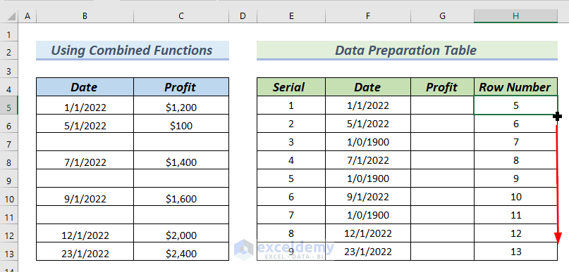
- Drag down the formula with the Fill Handle tool.
The complete Row Number column is filled.
![]()
Step 4 – Updating Formula in Cell H5
In cells H7, H9, and H11, we do not want Row Number 7, 9, or 11. For instance, we want 8 in cell H7 instead of 7, because cells B7, B9, and B11 have blank cells. We want the Row Number to skip these blank cells and update.
- Enter the following formula in cell H5:
=AGGREGATE(15,3,ROW($B$5:$B$13)/($B$5:$B$13<>""),E5)![]()
Formula Breakdown
- AGGREGATE(15,3,ROW($B$5:$B$13)/($B$5:$B$13<>””),E5) → the AGGREGATE function has multiple options for avoiding hidden rows along with error values.
- 15 → is the SMALL function_num.
- 3 → is the options that ignore hidden rows, error values, and nested SUBTOTAL and AGGREGATE functions.
- ROW($B$5:$B$13)/($B$5:$B$13<>””) → the ROW function returns the array for the AGGREGATE function.
- E5 → is the ref_1.
- AGGREGATE(15,3,ROW($B$5:$B$13)/($B$5:$B$13<>””),E5) → becomes
- Output: 5
- Explanation: 5 is the Row Number in cell H5.
- Press ENTER to return the result in cell H5.
- Drag down the formula with the Fill Handle tool.
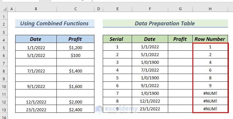
The values 7, 9, and 11 are missing in the Row Number column. The Row Number is now updated and blank cells are ignored.
![]()
Step 5 – Modifying Formula in Cell H5 by Using ROWS Function
Now we replace E5 in the formula in cell H5 with a formula written with the ROWS function to remove the Serial column from our Data Preparation Table. As a result, the Row Number will no longer depend on the Serial column.
- Enter the following formula in cell H5:
=AGGREGATE(15,3,ROW($B$5:$B$13)/($B$5:$B$13<>""),ROWS($B$5:B5))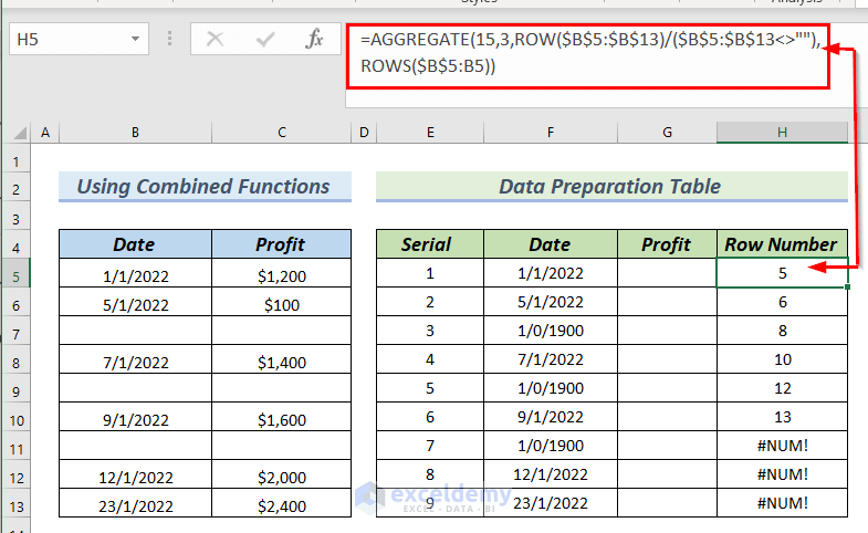
Formula Breakdown
- AGGREGATE(15,3,ROW($B$5:$B$13)/($B$5:$B$13<>””),ROWS($B$5:B5)) → the AGGREGATE function has multiple options for avoiding hidden rows along with error values.
- 15 → is the SMALL function_num.
- 3 → is the options that ignore hidden rows, error values, and nested SUBTOTAL and AGGREGATE functions.
- ROW($B$5:$B$13)/($B$5:$B$13<>””) → the ROW function returns the array for the AGGREGATE function.
- ROWS($B$5:B5 → the ROWS function returns the ref_1.
- AGGREGATE(15,3,ROW($B$5:$B$13)/($B$5:$B$13<>””),ROWS($B$5:B5)) → becomes
- Output: 5
- Explanation: 5 is the Row Number in cell H5.
- Press ENTER to return the result in cell H5.
- Drag down the formula with the Fill Handle tool.
![]()
The values are the same in the Row Number column, however the formula is different.
![]()
Step 6 – Changing Formula in Cell H5 to Number Rows Serially
The Row Number column starts from 5. However, we want the Row Number column to start from 1, and they must continue serially.
- Enter the following formula in cell H5:
=AGGREGATE(15,3,ROW($B$5:$B$13)-ROW($B$4)/($B$5:$B$13<>""),ROWS($B$5:B5))
Formula Breakdown
AGGREGATE(15,3,ROW($B$5:$B$13)-ROW($B$4)/($B$5:$B$13<>””),ROWS($B$5:B5)) → the AGGREGATE function has multiple options for avoiding hidden rows along with error values.
- 15 → is the SMALL function_num .
- 3 → is the options that ignore hidden rows, error values, and nested SUBTOTAL and AGGREGATE functions.
- ROW($B$5:$B$13)-ROW($B$4)/($B$5:$B$13<>””)→ returns the array for the AGGREGATE function.
- ROWS($B$5:B5 → the ROWS function returns the ref_1.
- AGGREGATE(15,3,ROW($B$5:$B$13)-ROW($B$4)/($B$5:$B$13<>””),ROWS($B$5:B5)) → becomes
- Output: 1
- Explanation: 1 is the Row Number in cell H5.
- Press ENTER to return the result in cell H5.
- Drag down the formula with the Fill Handle tool.
![]()
The Row Number now starts from 1 and goes serially.
Hence, the Row Number is the complete serial number for the INDEX function.
Step 7 – Copying Formula from Cell H5
We will copy the formula from cell H5 and paste the copied formula in cell F5:
=INDEX($B$5:$B$13,E5)Here we replace the cell reference E5 with the copied formula, which will end the dependence of the Date column on the Serial column.
- Copy the formula of cell H5. Simply select the formula and press CTRL+C to copy the formula.
![]()
Replace E5 from the formula of cell F5 by pasting the copied formula. The new formula becomes:
=INDEX($B$5:$B$13,AGGREGATE(15,3,ROW($B$5:$B$13)-ROW($B$4)/($B$5:$B$13<>""),ROWS($B$5:B5)))![]()
Formula Breakdown
- INDEX($B$5:$B$13,AGGREGATE(15,3,ROW($B$5:$B$13)-ROW($B$4)/($B$5:$B$13<>””),ROWS($B$5:B5))) → the INDEX function returns the value of an item in an array or table that are chosen by the indexes of a column and row number.
- $B$5:$B$13 → is the array.
- AGGREGATE(15,3,ROW($B$5:$B$13)-ROW($B$4)/($B$5:$B$13<>””),ROWS($B$5:B5)) → is the specified row number.
- INDEX($B$5:$B$13,AGGREGATE(15,3,ROW($B$5:$B$13)-ROW($B$4)/($B$5:$B$13<>””),ROWS($B$5:B5))) becomes
- Output: 01-01-2022
- Explanation: 01-01-2022 is the Date in cell F5.
We will also use the IFERROR function in the formula of cell F5 to ignore any sort of error.
The formula becomes:
=IFERROR(INDEX($B$5:$B$13,AGGREGATE(15,3,ROW($B$5:$B$13)-ROW($B$4)/($B$5:$B$13<>""),ROWS($B$5:B5))),"")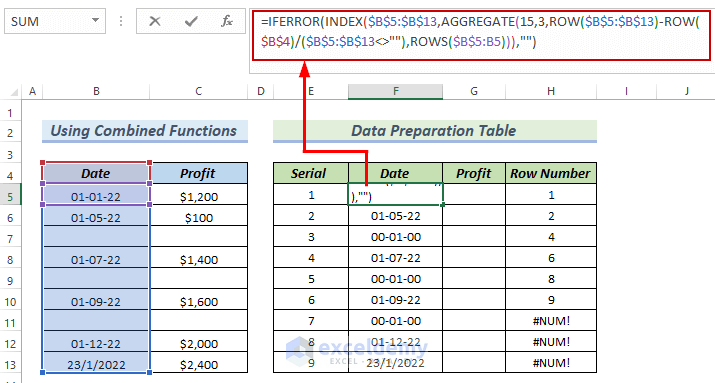
Formula Breakdown
- IFERROR(INDEX($B$5:$B$13,AGGREGATE(15,3,ROW($B$5:$B$13)-ROW($B$4)/($B$5:$B$13<>””),ROWS($B$5:B5))),””) → the IFERROR function ignores the error present in a formula.
- IFERROR(INDEX($B$5:$B$13,AGGREGATE(15,3,ROW($B$5:$B$13)-ROW($B$4)/($B$5:$B$13<>””),ROWS($B$5:B5))),””) → the IFERROR function ignores the error present in a formula → becomes
-
- Output: 01-01-2022
- Explanation: 01-01-2022 is the Date in cell F5.
- Press ENTER.
You can see the result in cell H5.
- Drag down the formula with the Fill Handle tool.
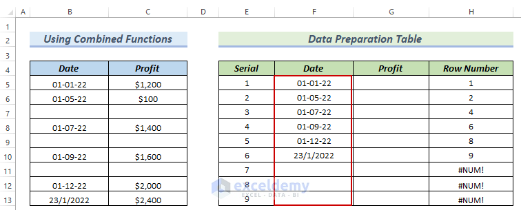
![]()
The Date column now ignores the blank cells.
Step 8 – Deleting Serial and Row Number Columns
In this step, we will delete the Row Number and Serial columns, because our Date column does not depend on these columns anymore.
- Select the entire Row Number column. Simply click on Column H to select the Row Number column.
- Right-click on it.
- Select Delete from the Context Menu.
![]()
- Repeat the process to delete the Serial column as well.
The Data Preparation Table now contains only the Date and Profit columns.
Step 9 – Completing Profit Column
We complete the Profit column by using the combination of INDEX and MATCH functions.
- Enter the following formula in cell F5:
=INDEX($C$5:$C$13,MATCH(E5,$B$5:$B$13,0))![]()
Formula Breakdown
- INDEX($C$5:$C$13,MATCH(E5,$B$5:$B$13,0)) → The INDEX function returns the value of an item in an array or table that is chosen by the indexes of the column and row number.
- $C$5:$C$13 → is the array.
- MATCH(E5,$B$5:$B$13 → the MATCH function returns the specified row_number.
- 0 means an exact match.
- INDEX($C$5:$C$13,MATCH(E5,$B$5:$B$13,0)) → becomes
- Output: 1200
- Explanation: 1200 is the Profit of cell F5.
- Press ENTER to return the result in cell H5.
- Drag down the formula with the Fill Handle tool.
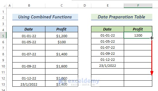
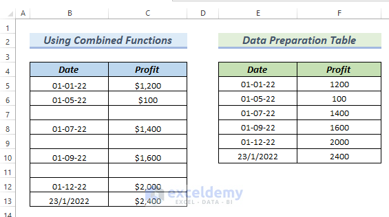
As a result, you can see the complete Profit column.
![]()
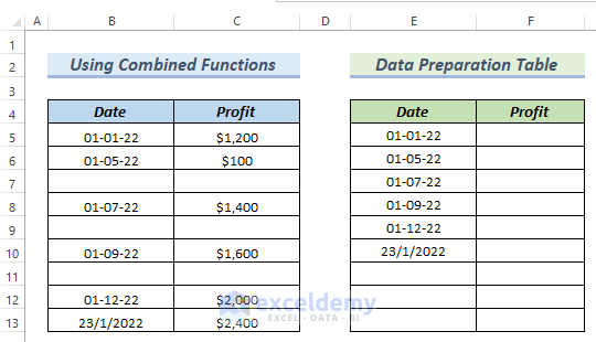
- Delete the last three columns of the Data Preparation Table as they do not contain any values.
The Data Preparation Table has no blank cells.
![]()
Step 10 – Inserting Bar Chart
Now we can insert a Bar chart using the following dataset.
- Follow Step 1 of Method 1 to insert the Bar chart and edit the chart title.
The Bar Chart ignores blank cells.
Read More: How to Create Bar Chart with Multiple Categories in Excel
Download Practice Workbook
Related Articles
- Excel Stacked Bar Chart with Subcategories
- How to Create Stacked Bar Chart with Line in Excel
- How to Plot Stacked Bar Chart from Excel Pivot Table
- How to Create Stacked Bar Chart with Dates in Excel
<< Go Back to Excel Bar Chart | Excel Charts | Learn Excel
Get FREE Advanced Excel Exercises with Solutions!
