Method 1 – Creating a Stacked Bar Chart with Dates in Excel
Steps:
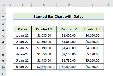
- Input the dates in the cell range B5:B10 and sales of different products of the corresponding date in the cell range C5:E10. Variables on the X-axis are represented by row headers, while variables on the Y-axis are represented by column headers.
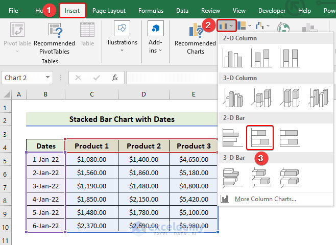
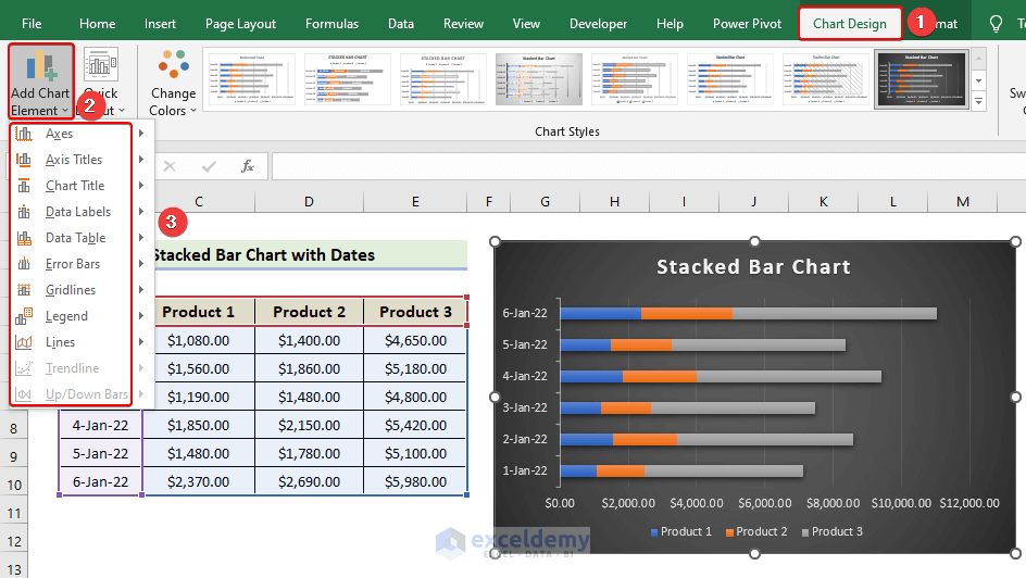
- Select the range of the cells B5:E10.
- In the Insert tab, click on the drop-down arrow of the Insert Column or Bar Chart from the Charts group.
- Choose the Stacked Bar Chart.
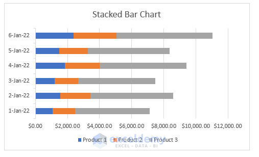
- You will get the following stacked bar chart.
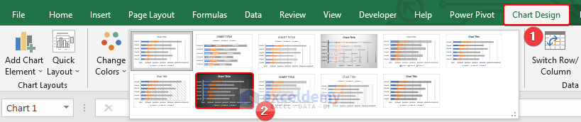
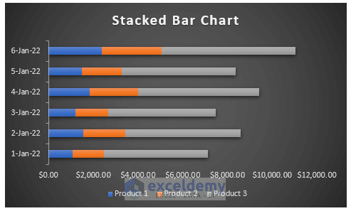
- To modify the chart style, select Chart Design and select your desired Style 8 option from the Chart Styles group.
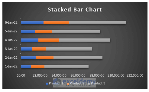
- You will get the following bar chart.
To add graph elements:
- In Quick Elements, some elements have already been added or removed. But you can manually edit the graph to add or remove any chart elements using the Add Chart Element option.
- Click on the Add Chart Element to see a list of elements.
- Click on them one by one to add, remove, or edit.
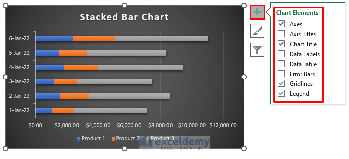
Alternatively, you can find the list of chart elements by clicking the Plus (+) icon from the right corner of the chart.
- Mark the elements to add or unmark the elements to remove.
- You will find an arrow on the element, where you will find other options to edit the elements.
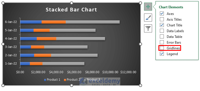
- If you want to remove the gridline from the chart, uncheck the Gridlines from the Chart Elements icon options.
- You will get the following stacked bar chart with dates.
Read More: How to Create Stacked Bar Chart with Negative Values in Excel
Method 2 – Creating a 100% Stacked Bar Chart with Dates in Excel
Steps:
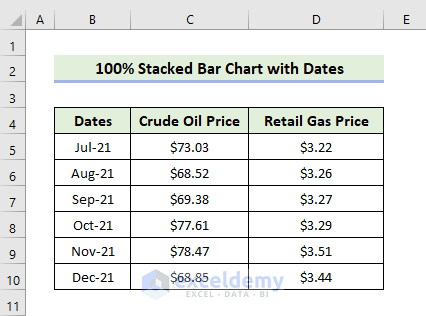
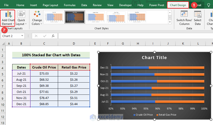
- Input the dates in the call range B5:B10 and sales of crude oil and retail gas of the corresponding date in the cell range C5:D10. Variables on the X-axis are represented by row headers, while variables on the Y-axis are represented by column headers.
- Select the range of the cells B5:D10.
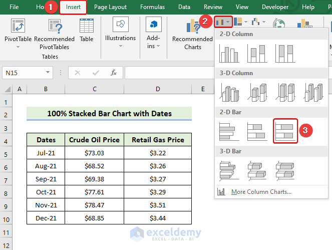
- In the Insert tab, click on the drop-down arrow of the Insert Column or Bar Chart from the Charts group.
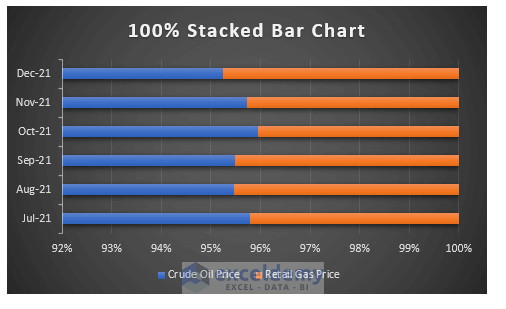
- Choose the 100% Stacked Bar Chart.
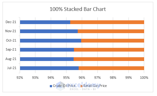
- You will get the following stacked bar chart.
- To modify the chart style, select Chart Design and select your desired Style 8 option from the Chart Styles group.

- You will get the following bar chart.
To add graph elements:
- In Quick Elements, some elements have already been added or removed. But you can manually edit the graph to add or remove any chart elements using the Add Chart Element option.
- You will see a list of elements after clicking on the Add Chart Element.
- Click on them one by one to add, remove, or edit.
Alternatively, you can find the list of chart elements by clicking the Plus (+) icon from the right corner of the chart.
- Mark the elements to add or unmark the elements to remove.
- You will find an arrow on the element, where you will find other options to edit the elements.
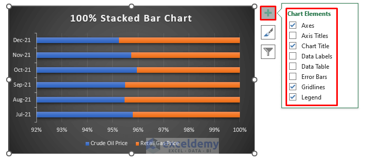
Now, we can customize the 100% stacked bar chart as you require by editing the Chart Elements. To remove the gridline, you need to uncheck the Gridlines. To add axis titles, check the Axis Titles from the Chart Elements and rename the axis based on your dataset.
Read More: How to Create Stacked Bar Chart for Multiple Series in Excel
Method 3 – Creating a 3-D Stacked Bar Chart with Dates in Excel
Steps:
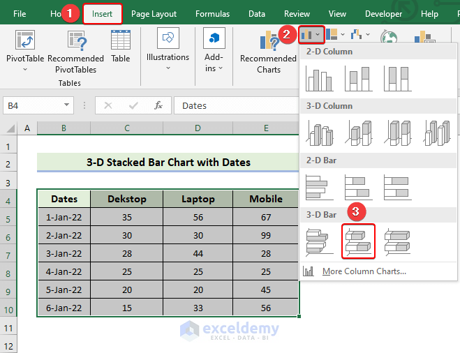
- Input the dates in cell range B5:B10 and the number of sales of laptops, mobile, and desktops of the corresponding date in cell range C5:E10. Variables on the X-axis are represented by row headers, while variables on the Y-axis are represented by column headers.
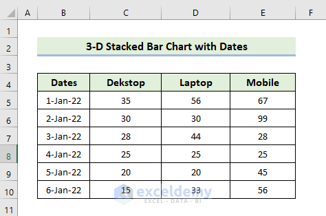
- Select the range of the cells B5:E10.
- In the Insert tab, click on the drop-down arrow of the Insert Column or Bar Chart from the Charts group.
- Choose the 3-D Stacked Bar Chart.
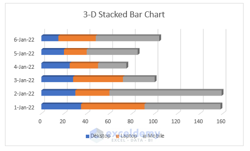
- You will get the following 3-D stacked bar chart.
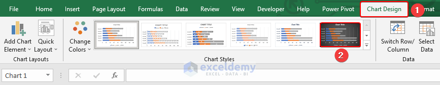
- To modify the chart style, select Chart Design and select your desired Style 6 option from the Chart Styles group.
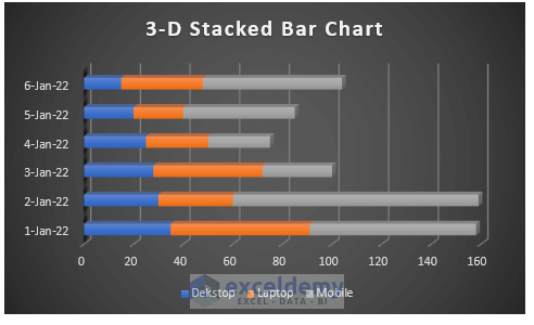
- You will get the following bar chart.
To add graph elements:
- In Quick Elements, some elements have already been added or removed. But you can manually edit the graph to add or remove any chart elements using the Add Chart Element option.
- After clicking on the Add Chart Element, you will see a list of elements.
- Click on them individually to add, remove, or edit.
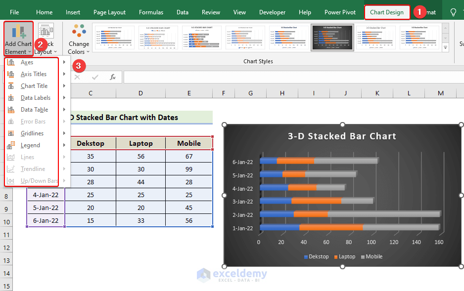
Alternatively, you can find the list of chart elements by clicking the Plus (+) icon from the right corner of the chart.
- Mark the elements to add or unmark the elements to remove.
- You will find an arrow on the element, where you will find other options to edit the elements.
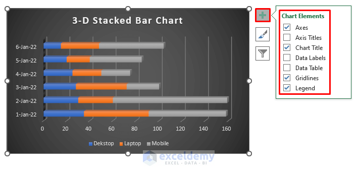
Now, we can customize the 3-D stacked bar chart as you require by editing the Chart Elements. To remove the gridline, you need to uncheck the Gridlines. To add axis titles, check the Axis Titles from the Chart Elements and rename the axis based on your dataset.
Read More: How to Create Stacked Bar Chart with Line in Excel
Things to Remember
✎ Before inserting a stacked bar chart, select anywhere in the dataset. The rows and columns will need to be manually added otherwise.
✎ Avoid stacked charts when working with a large dataset since they will create confusing graph information.
✎ If you want to switch rows and columns remember that before switching rows and columns, ensure they are all selected.
Download the Practice Workbook
Download this workbook to practice.
Related Articles
- How to Make a Stacked Bar Chart in Excel
- Excel Stacked Bar Chart with Subcategories
- How to Plot Stacked Bar Chart from Excel Pivot Table
- How to Create Bar Chart with Multiple Categories in Excel
- How to Ignore Blank Cells in Excel Bar Chart
<< Go Back to Stacked Bar Chart in Excel | Excel Bar Chart | Excel Charts | Learn Excel
Get FREE Advanced Excel Exercises with Solutions!
