Here’s an overview of the dataset we’ll be using to show how to sort bar chart without sorting data in excel.
Step 1 – Use RANK Function to Sort Data
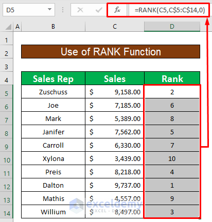
- Select cell D5.
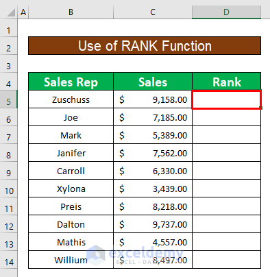
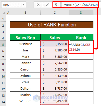
- Enter the following RANK function.
=RANK(C5,C$5:C$14,0)C5 is the number of the RANK function, C$5:C$14 is the ref of the RANK function, and 0 is the Descending order. We use the dollar ($) sign for the absolute reference of a cell.
- Press ENTER to get 2 which is the output of the RANK function.
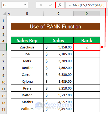
- AutoFill the RANK function to the rest of the cells in column C.
Read More: How to Make a Bar Graph Comparing Two Sets of Data in Excel
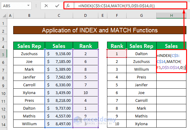
Step 2 – Combine INDEX and MATCH Functions to Sort in Ascending Order
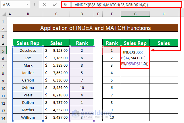
- Select cell D5 and enter the following INDEX and MATCH functions.
=INDEX(B$5:B$14,MATCH(F5,D$5:D$14,0))Formula Breakdown:
- Inside the MATCH function, F5 is the lookup_value, D$5:D$14 is the lookup_array, and 0 is used for the Exact match.
- Inside the INDEX function, B$5:B$14 is the reference, and MATCH(F5,D$5:D$14,0) is the row_num of the INDEX.
- We use the dollar ($) sign for the absolute reference of a cell.
- Press ENTER to get Dalton as the output of the INDEX and MATCH functions.
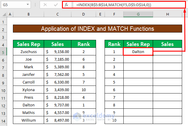
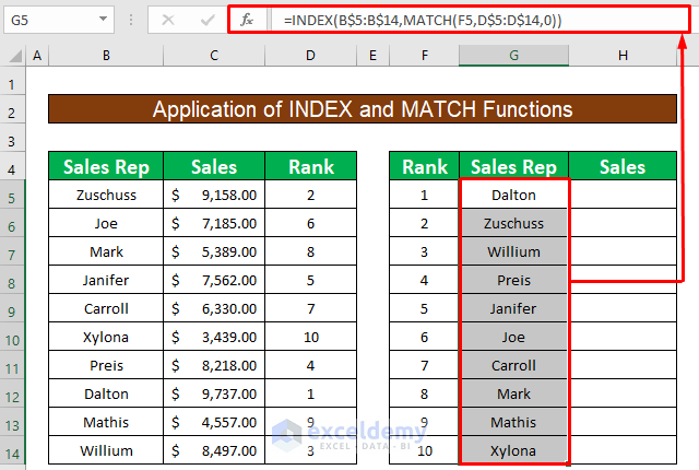
- AutoFill to the rest of the cells in column G.
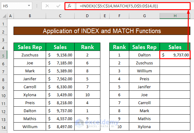
- Select cell H5 and enter the following INDEX and MATCH functions.
=INDEX(C$5:C$14,MATCH(F5,D$5:D$14,0))Formula Breakdown:
- Inside the MATCH function, F5 is the lookup_value, D$5:D$14 is the lookup_array, and 0 is used for the Exact match.
- Inside the INDEX function, C$5:C$14 is the reference, and MATCH(F5,D$5:D$14,0) is the row_num of the INDEX.
- We use the dollar ($) sign for the absolute reference of a cell.
- Press ENTER to get $9,737.00 as a return for the INDEX and MATCH functions.
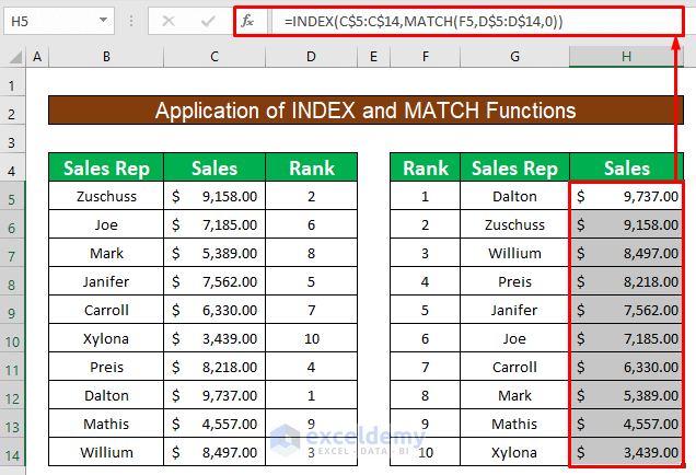
- AutoFill the rest of the cells in column H.
Read More: How to Show Difference Between Two Series in Excel Bar Chart
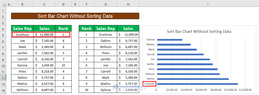
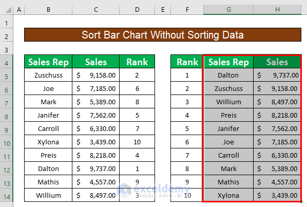
Step 3 – Create Bar Chart Without Sorting Data
- Select data ranging from G4 to H15.
- From Insert ribbon, go to,
Insert → Charts → 2-D Bar
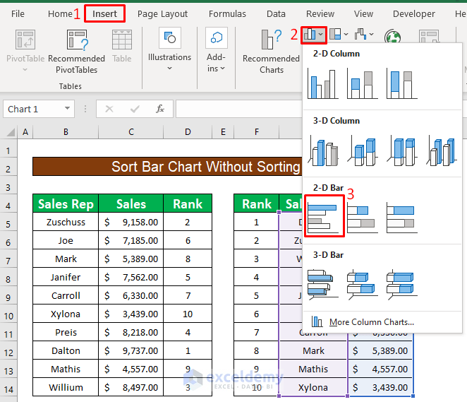
- You will be able to create a 2-D Bar chart without sorting data.
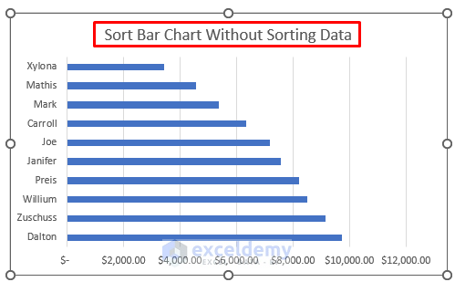
- To check if bar chart works, change the sale value of Zuschuss from $9,158.00 to $11,000.00. Notice that the 2-D Bar chart sorts automatically by changing the data.
Read More: How to Change Bar Chart Width Based on Data in Excel
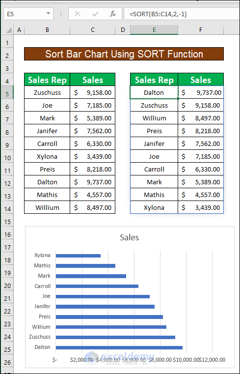
Alternative: Sort Bar Chart Using Excel SORT Function
- Select a cell (e.g., E5) and use the given formula to sort the entire dataset based on the sales column:
=SORT(B5:C14,2,-1)B5:D14 is the range of your data. “2” specifies the 2nd column to sort (sales column in this case), and “-1” indicates descending order.
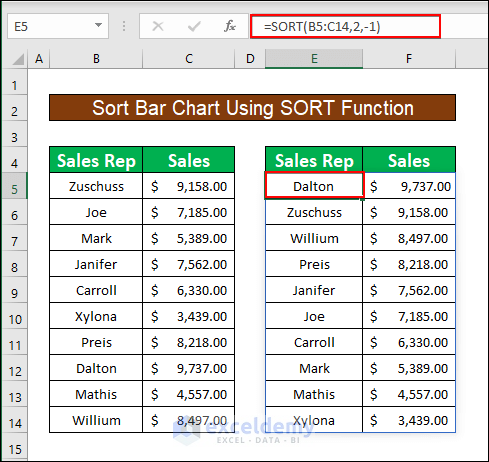
- The sorted data is in cell range E5:F14.
- To create the sorted bar chart, select the first cell (e.g. E5) of sorted data, go to the Insert tab and select 2-D Bar Chart.
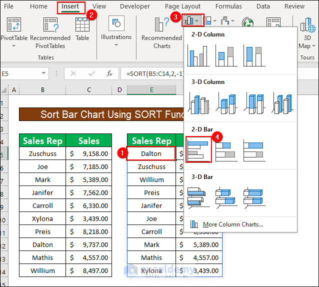
- You will get the Bar chart based on the sorted sales data.
Things to Remember
#N/A! error happens when the formula or a function in the formula fails to find the referenced data.
#DIV/0! error happens when a value is divided by zero(0) or the cell reference is blank.
Download Practice Workbook
Related Articles
- How to Make a Bar Graph with Multiple Variables in Excel
- How to Make a Bar Graph in Excel with 2 Variables
- How to Make a Bar Graph in Excel with 3 Variables
- How to Make a Bar Graph in Excel with 4 Variables
- How to Make a Percentage Bar Graph in Excel
- How to Show Number and Percentage in Excel Bar Chart
- Excel Bar Chart Side by Side with Secondary Axis
<< Go Back to Excel Bar Chart | Excel Charts | Learn Excel
Get FREE Advanced Excel Exercises with Solutions!

What if two of your sales values are identical resulting in two same rankings?
Thanks, KYLE, for your query. If there are identical values, then it will give same Rank. Also, the RANK function will skip one Rank. For your better understanding, I’m changing the sales value of Janifer to $9158. So, Zuschuss and Janifer get the same rank (2nd). Thus, the 3rd rank will be missed. Here, you must re-write the Rank of F7 cell to “2” and change the array for INDEX-MATCH function using in G7 an H7 cell. Basically, you need to set the array without Zuschuss information. Below, I have attached the whole scenario.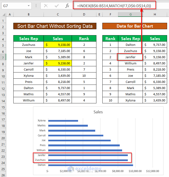
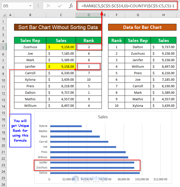
There is another way, if you want to get unique Rank for all. Like Zuschuss comes first than Janifer so Zuschuss will get 2nd rank and Janifer will get 3rd rank. In this case, you just need to change the formula in D column given below: =RANK(C5,$C$5:$C$14,0)+COUNTIF($C$5:C5,C5)-1
You don’t need to change the array of INDEX-MATCH function.
Regards
Musiha Mahfuza Mukta| Team Exceldemy
Hi Md. Abdur Rahim Rasel, first, I wanted to thanks for your excellent website and the amazing help you provide – it is one of the best all around.
Second, I tried your approach to sort bar chart without sorting the data and every single time, either using your example excel or my own file, the results after doing the INDEX, MATCH, it is #N/A.
Thank you, CARLOS for your comment. You have to use the correct array (Sales Rep
or B5:B14) in INDEX function and Rank Column (D5:D14) in MATCH function. Also, while using the Fill Handle icon, you have to freeze both arrays. The most important part, you must write Rank 1,2,3.. manually in General format in F column.
There may have extra space or Apostrophe (‘) in the F column where you insert Rank numbers manually. You should remove all extra spaces.
You can see our article related MATCH function error. The link is: https://www.exceldemy.com/excel-match-function-not-working/#Case_1_NA_Error
For getting basic idea of INDEX-MATCH function you can see the examples from this article https://www.exceldemy.com/excel-index-match-example/
Still, you are facing the problem then please comment with your used formula and sample dataset.
Regards
Musiha Mahfuza Mukta| Team Exceldemy.