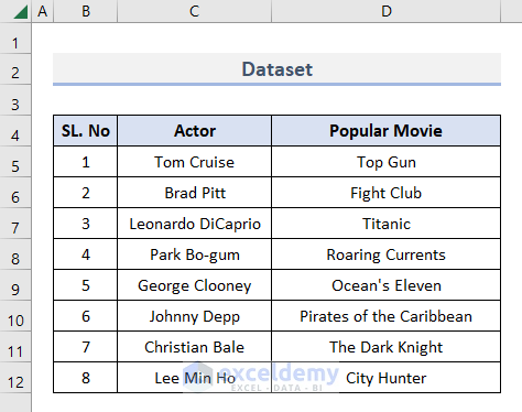
Let’s use a table that contains several actors from different film industries with one of their popular movies. We’ll find different values based on movie or actor names.
Method 1 – Use the MATCH Function to Find a Value in the Range
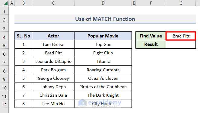
Let’s determine if an actor is present in the range.
- Add two fields Find Value and Result beside the table.
- Insert your required value in Cell G4.
- Insert this formula in Cell G5.
=IF(ISNUMBER(MATCH(G4,C5:C12,0)),"Found","Not Found")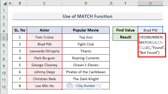
- Press Enter.
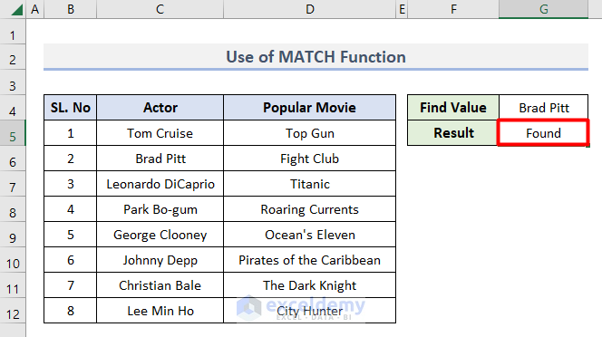
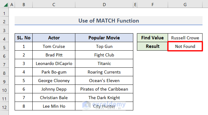
- You will see the output as Found because the finding value is preset in the dataset.
Here, the MATCH function checks whether the value is present in the Cell range C5:C12. When it doesn’t get the character within the string it returns #N/A error. Alongside this, the ISNUMBER function checks if the value in Cell G4 is numeric or not. Lastly, the IF function makes a comparative statement among them.
- If we search for a value that is not in the range, the formula will return Not Found.
- If you want the position of the value, apply this formula.
=MATCH(G4,C5:C12,0)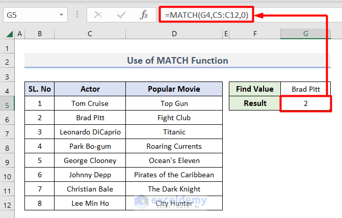
We have set Cell G4 as the lookup_value in the MATCH function. Then C5:C12 is the range and 0 for the exact match. As a result, you can see Brad Pitt is 2nd in our table, and the formula returned that number.
Method 2 – Combine IF & COUNTIF Functions to Search for a Value in a Range
- Use this formula in Cell G5.
=IF(COUNTIF(C5:C12,G4)>0,"Found","Not Found")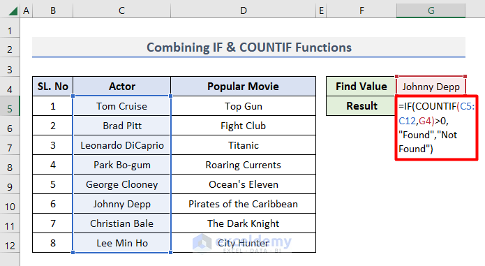
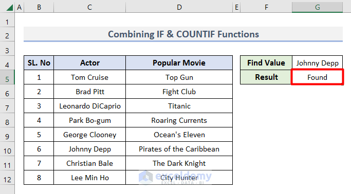
- Press Enter and you will get the result.
In this formula, within COUNTIF(C5:C12,G4)>0, C5:C12 is the range and G4 is the value to find. Since the COUNTIF function counts cells based on criteria, it will count the cells from the C5:C12 range based on G4. If it finds the value, the result will be greater than 0. If the value is greater than 0, it means the value is found in the range. And the if_true_value (Found) will be the result.
Method 3 – Find a Value in a Range with the VLOOKUP Function in Excel
- Insert this formula in Cell G5.
=VLOOKUP(G4,C5:C12,1,0)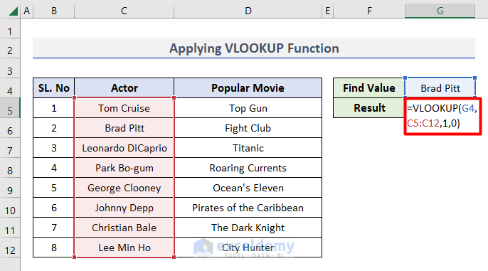
- We will get the value itself as the result of our formula.

In the formula, G4 is the lookup_value and C5:C12 is the range, 1 is the column_num, and 0 is for an exact match. This will neither deliver the position nor a Boolean value, rather it will retrieve the value corresponding to the findings.
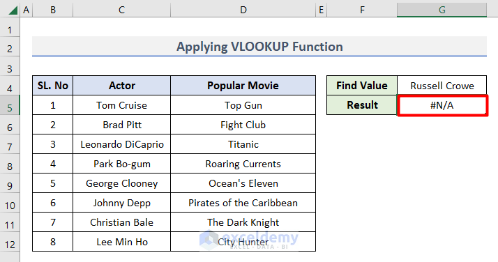
- If we search for something that is not in the range the formula will provide a #N/A error.
- We can use the IFNA function to remove the error. Use this formula instead.
=IFNA(VLOOKUP(G4,C5:C12,1,0),"Not Found")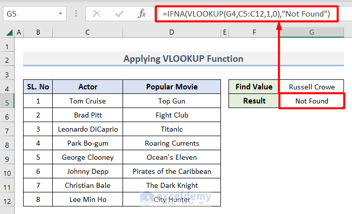
The IFNA function checks whether the supplied value in Cell G4 evaluates the Excel #N/A error or not. Therefore it replaces the result for #N/A. We wrapped up the VLOOKUP with IFNA and set “Not Found” as ifna_value. So, when it does not find a value in the range, it will provide “Not Found” as a result.
- When the value is in the range, the standard VLOOKUP function result will be the final output.

Read More:
- How to Find Last Row with a Specific Value in Excel
- Excel Find Last Column With Data
- How to Find Highest Value in Excel Column
How to Find and Return Value in Range in Excel
Let’s say we want to derive the name of the movie by finding the actor’s name in the range.
- Use this formula in Cell G5.
=INDEX(D5:D12,MATCH(G4,C5:C12,0))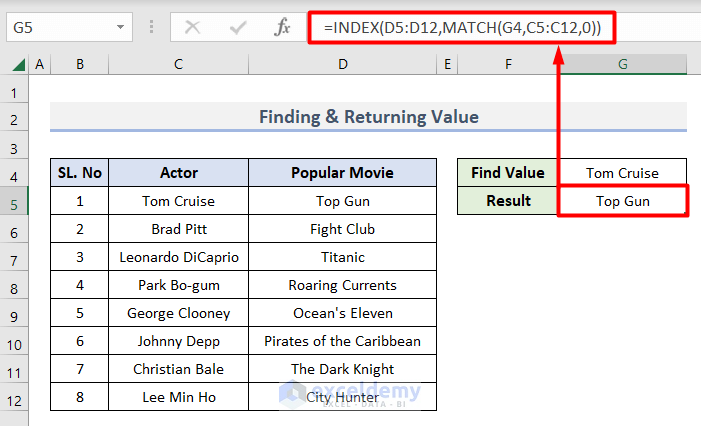
We have seen MATCH return the position of the matched value, and then INDEX uses that position value to return the value from the Cell range D5:D12.
- Alternatively, you can use this formula:
=VLOOKUP(G4,C5:D12,2,0)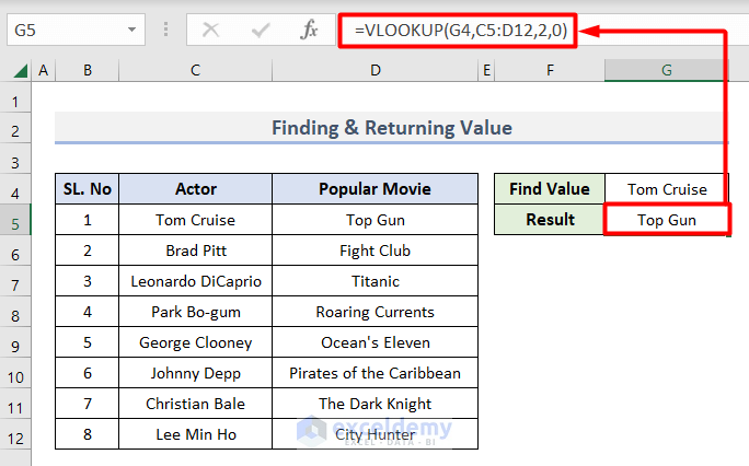
Here we have inserted almost the entire table (except the SL. No column) as the range. The column_num_index is 2, which means depending on the match the value will be fetched from the 2nd column of the range. And the second column contains the movie’s name.
- For Excel 365, you can also use this formula:
=XLOOKUP(G4,C5:C12,D5:D12)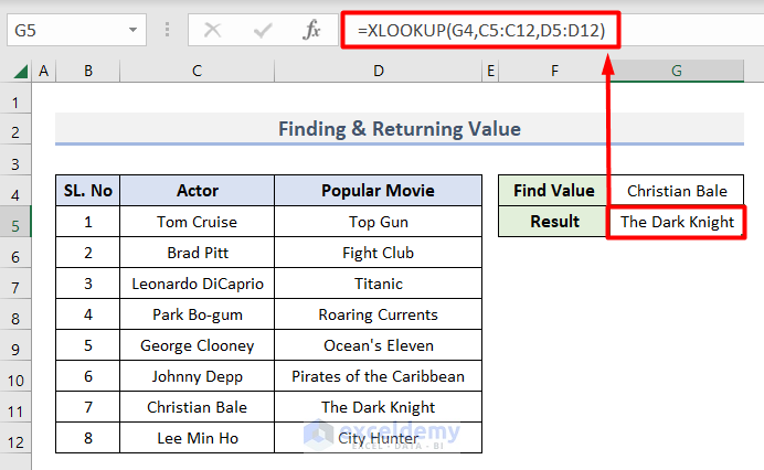
In this formula, within the XLOOKUP function, we have inserted the search value (G4), then the lookup range (C5:C12), and finally the range (D5:D12) from where we want the output.
- Modify the previous formula to get “Not Found” as a result if you don’t get a match:
=XLOOKUP(G4,C5:C12,D5:D12,"Not Found")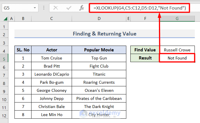
Read More:
- How to Find Lowest Value in an Excel Column
- How to Use Excel Formula to Find Last Row Number with Data
- How to Find Multiple Values in Excel
Download the Practice Workbook
Excel Find Value in Range: Knowledge Hub
- How to Find First Value Greater Than in Excel
- How to Find First Occurrence of a Value in a Range in Excel
- How to Find Value in Column in Excel
- How to Find First Occurrence of a Value in a Column in Excel
- How to Check If a Value is in List in Excel
- Find Last Value in a Range in Excel
- [Solved!] CTRL+F Not Working in Excel
- Lookup Value in Column and Return Value of Another Column in Excel
- How to Find Top 5 Values and Names in Excel
- Find Text in Excel Range and Return Cell Reference
- How to Search Text in Multiple Excel Files
- How to Get Top 10 Values Based on Criteria in Excel
- How to Create Top 10 List with Duplicates in Excel
<< Go Back to Excel Range | Learn Excel
Get FREE Advanced Excel Exercises with Solutions!

This is an excellent and very helpful article; thanks! But what I need is not H4 but to be able to loop through one list to see if its values are in another list. For example, my “Actor” column would be one long email list “All” and my “Movie” column would be a shorter list “Some”, and I need to see if the values in the “All” list are in the “Some” list.