There are a few reasons for which you might want to ignore blank axis labels in an Excel Chart. Such as, it can make the chart look cleaner and less cluttered, make it easier to see the data that is being plotted, to make it easier to compare data points on the chart. However, you need to create some extra helper columns to make your Excel Chart ignore the blank axis labels. In this article, I will guide you to ignore blank axis labels in an Excel Chart with easy steps. So without having any further discussion, let’s get started.
Ignore Blank Axis Labels in Excel Chart: with Easy Steps
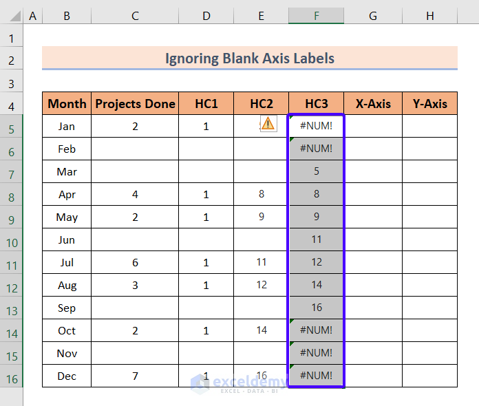
I’m going to use the following Projects Tracking Record to show you ignore the blank axis labels in the Excel chart. The following dataset has two columns; one comprising the month names and the other has the corresponding number of projects completed.
![]()
Step-1: Creating First Helper Column (HC1)
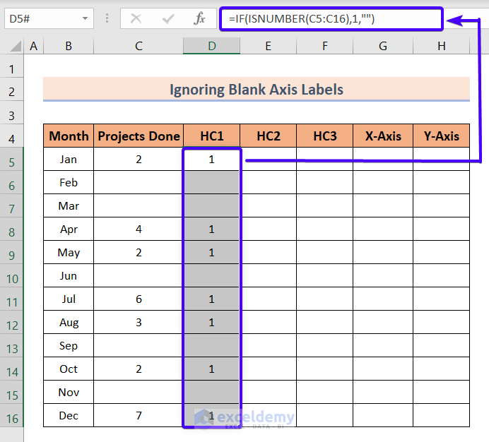
In the first helper column, I will use a formula to return 1 for the months that have a minimum of 1 completed project.
To do that,
❶ Insert the following formula in cell D5.
=IF(ISNUMBER(C5:C16),1,"")❷ Then press ENTER.
Formula Breakdown
- The ISNUMBER function returns TRUE if the range C5:C16 has any number. Otherwise, it returns a FALSE.
- The IF function returns 1 when the ISNUMBER function returns a TRUE; otherwise, it returns an empty string.
Step-2: Creating Second Helper Column (HC2)
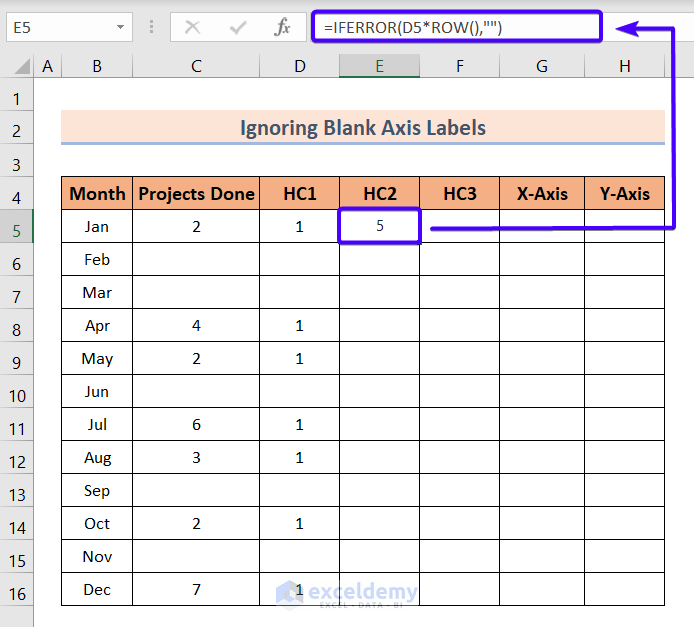
The second helper column is used to return the row index number of the months that a minimum of 1 project completion record.
For that,
❶ Insert the following formula in cell E5.
=IFERROR(D5#*ROW(),"")❷ Then press ENTER.
Formula Breakdown
- The ROW function returns the row index number of cell D5 if it has 1. If cell D5 contains a blank, the ROW function doesn’t return anything but an empty string.
- The IFERROR function returns a null value if the ROW function returns any type of error.
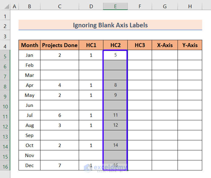
❸ Drag the Fill Handle from cell E5 to E16.
![]()
Finally, you will get the row index number of all the months that have a minimum of 1 project completion record.
Step-3: Creating Third Helper Column (HC3)
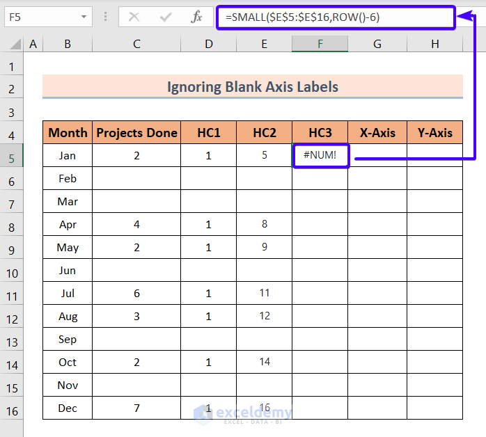
I will use the third helper column to arrange all the row index numbers from the second helper column in descending order.
Now follow the steps below:
❶ Insert the following formula in cell F5.
=SMALL($E$5:$E$16,ROW()-6)❷ Press ENTER.
Formula Breakdown
- ROW()-6 returns to the relative position number of the row index numbers to rank them.
- The SMALL function returns the row index number in the range $E$5:$E$16 from smallest to largest.
❸ Drag the Fill Handle icon from cell F5 to F16.
![]()
Finally, you will see the row index numbers from the second helper column are arranged together. The row index numbers are also sorted from the smallest to largest.
Step-4: Generating X-Axis Column
In the X-Axis column, I will use a formula to get only those months’ names that are not blanks.
For that,
❶ Insert the following formula in cell G5.
=IF(ISNUMBER(F5),INDEX($B$5:$B$16,MATCH(F5,$E$5:$E$16,0)),"")❷ Then press ENTER.
Formula Breakdown
- MATCH(F5,$E$5:$E$16,0): Here the MATCH function looks for matches between F5 and $E$5:$E$16. If it finds any matches, it returns 1; otherwise, it returns 0.
- INDEX($B$5:$B$16,MATCH(F5,$E$5:$E$16,0)): The INDEX function returns the name of the months from the range $B$5:$B$16 based on the matching results from the MATCH
- ISNUMBER(F5): The ISNUMBER function checks are cell F5 has a number or not.
- IF(ISNUMBER(F5),INDEX($B$5:$B$16,MATCH(F5,$E$5:$E$16,0)),””): The IF function returns value of INDEX($B$5:$B$16,MATCH(F5,$E$5:$E$16,0)), if the ISNUMBER function returns a TRUE; otherwise, it returns a null value.
![]()
❸ Now drag the Fill Handle icon from cell G5 to G16.
![]()
Finally, you will get all the months that are not blank in the Projects Done column.
![]()
Read More: How to Add Axis Titles in Excel
Step-5: Generating Y-Axis Column
In the column, Y-Axis, I will use a formula to return the number of projects from the column, Projects Done.
To do that,
❶ Insert the following formula in cell H5.
=VLOOKUP(G5,$B$5:$C$16,2,FALSE)❷ Then press ENTER.
Formula Breakdown
- G5 is the lookup_value.
- $B$5:$C$16 is the table_array.
- 2 is the column index number.
- FALSE refers to an exact match.
- VLOOKUP(G5,$B$5:$C$16,2,FALSE): The VLOOKUP function looks for an exact match between G5 and $B$5:$C$16. Then it returns values from the 2nd column of the range which is $C$5:$C$16.
![]()
❸ Now drag the Fill Handle icon from cell H5 to H16.
![]()
Finally, you will get all the numbers of projects completed from the column, Projects Done.
![]()
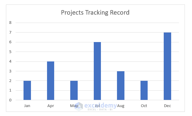
Step-6: Inserting a Column Chart
Now, it’s time to insert a chart based on the data in columns, X-Axis and Y-Axis.
For that,
❶ Select the range G7:H13.
❷ Now go to the Insert tab.
❸ Click on the Recommended Charts command in the Charts group.
![]()
Insert Chart dialog box will appear.
❹ Click on the Clustered Column chart type.
❺ Then hit OK.
![]()
Finally, you will get an Excel chart ignoring all the blank axis labels.
Read More: How to Add X and Y Axis Labels in Excel
Practice Section
You will get an Excel sheet like the following screenshot, at the end of the provided Excel file where you can practice all the topics discussed in this article.
![]()
Download Practice Workbook
You can download the Excel file from the following link and practice along with it.
Conclusion
I have discussed steps to ignore blank axis labels in Excel Chart. Please don’t hesitate to ask any questions in the comment section below. We will try to respond to all the relevant queries asap.
Related Articles
<< Go Back To Label Axis in Excel | Excel Chart Elements | Excel Charts | Learn Excel
Get FREE Advanced Excel Exercises with Solutions!
