There are several distinct Microsoft Excel functions for determining the average of integer values. Additionally, there is a quick non-formula way. This article shows 4 easy ways to find average with blank cells in Excel. We will discuss a brief summary of each technique in this tutorial, along with usage examples and best practices. Every function covered in this article is compatible with Excel 2007 through the latest Excel 365 version.
How to Find Average with Blank Cells in Excel: 4 Easy Ways
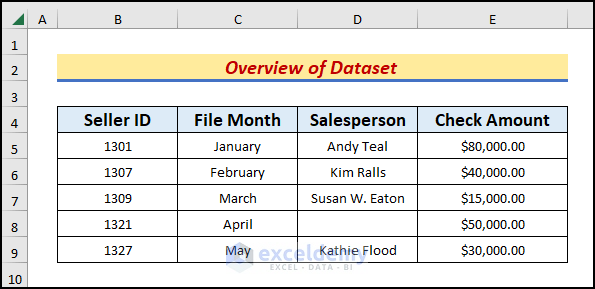
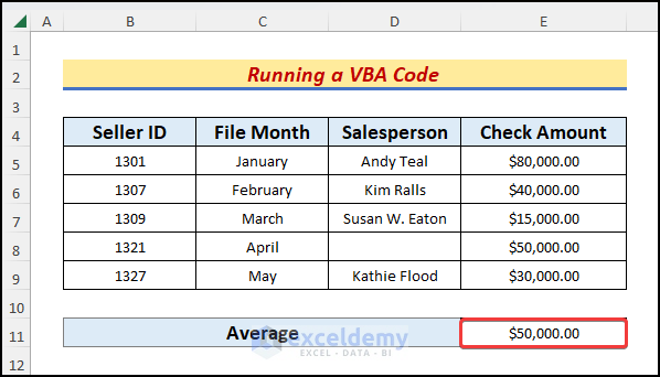
The average is determined by dividing the total of all the values by their number. It is the mean or middle value in a group of numbers in mathematics. However, if we wish to take the empty cells into account, we can use three functional methods and one VBA approach. To demonstrate, let’s take a dataset that represents the budget book of a sales company. See the picture below you will notice a blank cell in column D. In this tutorial, we will learn how to find the average of column E including the corresponding empty cells in column D.
1. Use AVERAGEIF Function to Find Average with Blank Cells in Excel
In the first step, we will use the AVERAGEIF function to average numbers with blank cells. The AVERAGEIF function determines an arithmetic mean from an array under a specified condition and returns it in a numerical value. Based on the corresponding column D, let’s find out the average of the column E.
Steps:
- Firstly, add a row named Average in row 11.
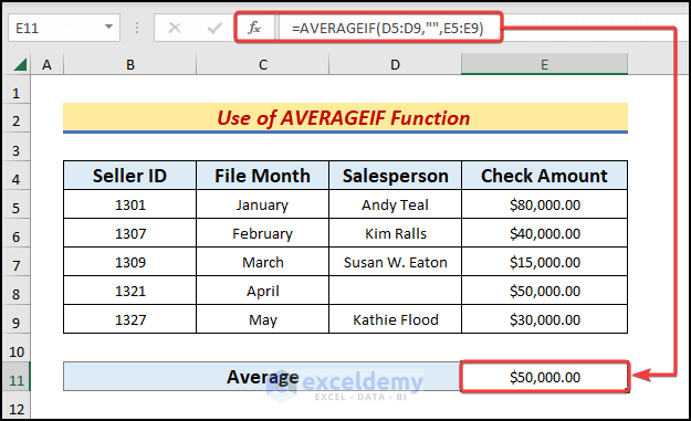
- Type the following formula in cell E11.
=AVERAGEIF(D5:D9,"",E5:E9)- Here, the AVERAGEIF function compares our selections to D5:D9.
- Furthermore, it decides which cells within the given range shall be averaged through “”.
- Finally, it calculates the average from the range E5:E9.
- Afterward, press the Enter or Tab keys to find the output as $50,000.00.
Read More: How to Average Only Visible Cells in Excel
2. Combine SUMPRODUCT and AVERAGE Functions to Find the Average with Zero Cells
The second method aims to adjoin the SUMPRODUCT and AVERAGE functions to count the average including the empty cells. The AVERAGE function under the Statistical function category returns the average of a given range. Furthermore, the SUMPRODUCT function takes one or more cell ranges as an argument and multiplies the corresponding values of all the ranges. Finally, returns the summation of the products.
Steps:
- To begin with, write the formula down in cell E11.
=SUMPRODUCT(AVERAGE(0+E5:E9))- Later, by pressing the Enter or Tab buttons, we get the output as $40,000.00.
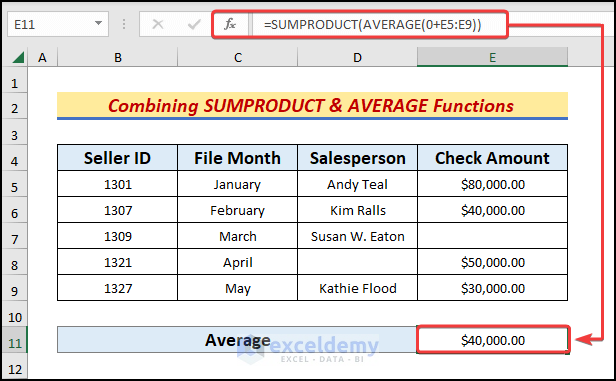
Hence, we get the average of the check amounts including blank cells.
Read More: How to Calculate Average Only for Cells with Values in Excel
3. Combine Excel SUM and ROWS Functions to Calculate Average Counting Null Cells
The objective of the third method is to combine the SUM and ROWS functions thoroughly to find the average taking the empty cells into account. The SUM function determines the summation of an array and returns an integer as an output. Alternatively, the ROWS function is a built-in Excel function under the LOOKUP & REFERENCE function category that returns the number of rows existing within a given array.
Steps:
- First, in cell E11, type the following formula.
=SUM(E5:E9)/ROWS(E5:E9)- Further, press the Enter or Tab keys to get an output of $40,000.00.
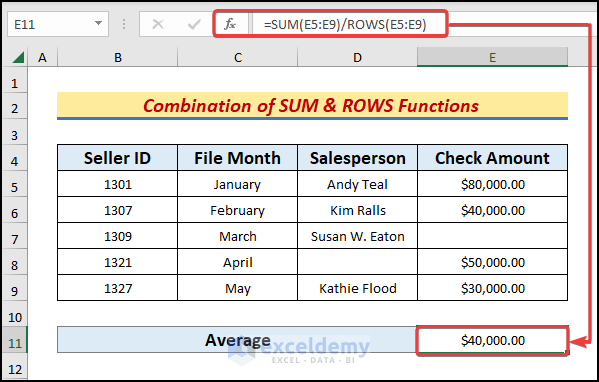
- As a result, the average pop-up in the display also counts the empty cell.
- ROWS(E5:E9) returns the total row numbers as 5.
- SUM(E5:E9) returns the summation of the range (E5:E9).
- SUM(E5:E9)/ROWS(E5:E9) finally divides the products to finally get the average.
4. Run VBA Code to Count Average Including Empty Cells in Excel
In our last method, we will run a VBA code to calculate the average with the blank cells. The VBA approach needs to use VBA Objects and specified parameters. Furthermore, we will also mention the specific worksheet names in the code. Let’s jump into the code to understand properly how the method works.
Steps:
- Go to the Developer tab and click the Visual Basic option.

- The Visual Basic window appears in the display.
- Tap the Insert tap and then Module to create a module box.
![]()
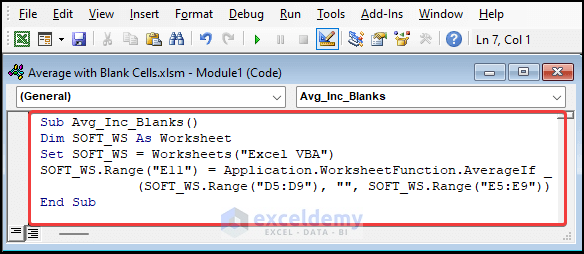
- In the module box, type the following VBA code correctly.
Sub Avg_Inc_Blanks()
Dim SOFT_WS As Worksheet
Set SOFT_WS = Worksheets("Excel VBA")
SOFT_WS.Range("E11") = Application.WorksheetFunction.AverageIf(SOFT_WS.Range("D5:D9"), "", SOFT_WS.Range("E5:E9"))
End Sub- After that, close the window to open the active sheet.
- Meanwhile, go to the Developer tab and tap Macros.
![]()
- The Macro dialog box pops up.
- Select the desired macro from the Macro name box and hit the Run button.
![]()
- Lastly, the average appears as $50,000.00 in cell E11.
- As Worksheet is a representation of all the worksheets of the workbook but excludes the chart sheets.
- Worksheets(“Excel VBA”) we input the active worksheet name here.
- Range represents an Object that makes sure that all the given ranges get declared.
Download Practice Workbook
Download this practice workbook to exercise while reading this article. It contains all the datasets in different spreadsheets for a clear understanding. Try it yourself while you go through the whole process.
Conclusion
In conclusion, we have discussed some easy ways to find the average with blank cells in Excel. Please leave any further queries or recommendations in the comment box below.
Related Articles
- How to Calculate Average of Multiple Columns in Excel
- How to Calculate Average of Multiple Ranges in Excel
- How to Average a Column in Excel
- How to Average Every Nth Row in Excel
- How to Find Average of Specific Cells in Excel
- How to Exclude a Cell in Excel AVERAGE Formula
- How to Fix Divide by Zero Error for Average Calculation in Excel
- How to Ignore #N/A Error When Getting Average in Excel
- [Fixed!] AVERAGE Formula Not Working in Excel
<< Go Back to Calculate Average in Excel | How to Calculate in Excel | Learn Excel
Get FREE Advanced Excel Exercises with Solutions!
