The Math & Trig functions in Excel are used for basic arithmetic, conditional sum & product, exponent & logarithm, and trigonometric ratios. Some math-related functions are found in the Statistical functions and Engineering functions categories. Here is an overview of the 51 most commonly used, listed alphabetically.
51 Mostly Used Math and Trig Functions in Excel
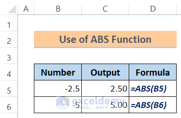
1. The ABS Function
- Function Objective:
The ABS function finds out the absolute value of a number.
- Syntax:
=ABS(number)
- Arguments Explanation:
| Argument | Required/Optional | Explanation |
|---|---|---|
| number | Required | A number |
- Return Parameter:
The absolute value of a number
Use of ABS Function:
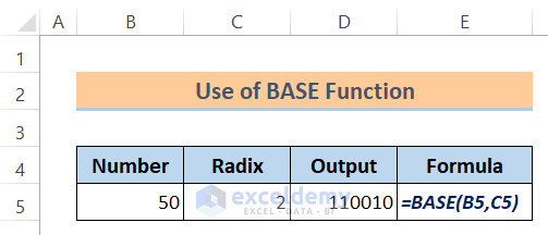
2. The BASE Function
- Function Objective:
The BASE function converts a number into a text representation with the given radix (base).
- Syntax:
=BASE(number, radix, [min_length])
- Arguments Explanation:
| Argument | Required/Optional | Explanation |
|---|---|---|
| number | Required | The number that you want to convert. |
| radix | Required | The base radix that you want to convert the number into. |
| [min_length] | Optional | The minimum length of the returned string. |
- Return Parameter:
Converts a number into a text representation with the given radix.
Use of BASE Function:
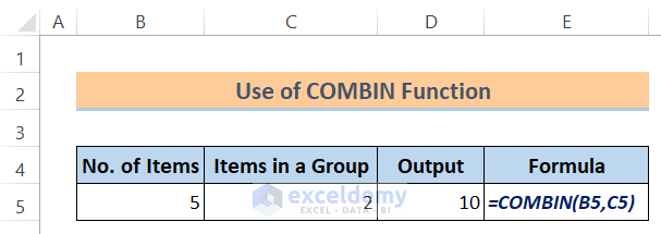
3. The COMBIN Function
- Function Objective:
The COMBIN function returns the number of combinations for a given number of items.
- Syntax:
=COMBIN (number, number_chosen)
- Arguments Explanation:
| Argument | Required/Optional | Explanation |
|---|---|---|
| number | Required | The number of items. |
| number_chosen | Required | The number of items in each combination. |
- Return Parameter:
To determine the total possible number of groups for a given number of items.
Use of COMBIN Function:
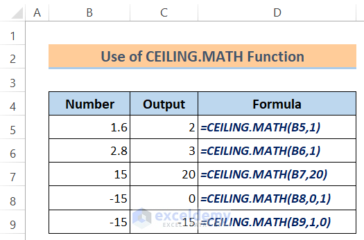
4. The CEILING.MATH/CEILING Function
- Function Objective:
The CEILING.MATH function is used to round a number up to the nearest integer or to the nearest multiple of significance.
- Syntax:
=CEILING.MATH (number, [significance], [mode])
- Arguments Explanation:
| Argument | Required/Optional | Explanation |
|---|---|---|
| number | Required | The number must be less than 9.99E+307 and greater than -2.229E-308. |
| significance | Optional | The multiple to which the number is to be rounded. |
| mode | Optional | For negative numbers, controls whether the number is rounded toward or away from zero. |
- Return Parameter:
Rounds a number up to the nearest integer or to the nearest multiple of significance.
Use of CEILING.MATH/CEILING Function:
5. The COS Function
- Function Objective:
The COS function is used to return the cosine of the given angle.
- Syntax:
=COS(number)
- Arguments Explanation:
| Argument | Required/Optional | Explanation |
|---|---|---|
| number | Required | The angle in radians. |
- Return Parameter:
Returns the cosine of the given angle.
Use of COS Function:

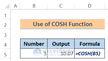
6. The COSH Function
- Function Objective:
The COSH function is used to return the hyperbolic cosine of a number.
- Syntax:
=COSH(number)
- Arguments Explanation:
| Argument | Required/Optional | Explanation |
|---|---|---|
| number | Required | A real number for which you want to find the hyperbolic cosine. |
- Return Parameter:
Returns the hyperbolic cosine of a number.
Use of COSH Function:
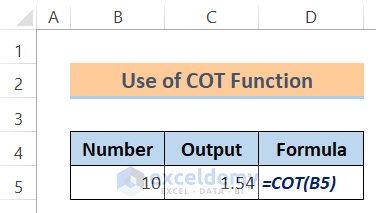
7. The COT Function
- Function Objective:
The COT function is used to return the cotangent of an angle specified in radians.
- Syntax:
=COT (number)
- Arguments Explanation:
| Argument | Required/Optional | Explanation |
|---|---|---|
| number | Required | The angle in radians for which we want the cotangent. |
- Return Parameter:
The cotangent of an angle is specified in radians.
Use of COT Function:
8. The COTH Function
- Function Objective:
The COTH function is applied to return the hyperbolic cotangent of a hyperbolic angle.
- Syntax:
=COTH(number)
- Arguments Explanation:
| Argument | Required/Optional | Explanation |
|---|---|---|
| number | Required | The angle in radians for which we want the hyperbolic cotangent. |
- Return Parameter:
The hyperbolic cotangent of a hyperbolic angle.
Use of COTH Function:

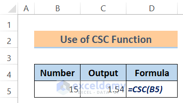
9. The CSC Function
- Function Objective:
The CSC function is used to return the cosecant of an angle specified in radians.
- Syntax:
=CSC(number)
- Arguments Explanation:
| Argument | Required/Optional | Explanation |
|---|---|---|
| number | Required | The angle in radians for which we want to calculate the cosecant. |
- Return Parameter:
The cosecant of an angle is specified in radians.
Use of CSC Function:
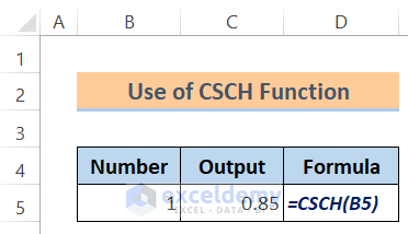
10. The CSCH Function
- Function Objective:
The CSCH function is applied to return the hyperbolic cosecant of an angle specified in radians.
- Syntax:
=CSCH(number)
- Arguments Explanation:
| Argument | Required/Optional | Explanation |
|---|---|---|
| number | Required | The angle in radians for which we want to calculate the hyperbolic cosecant. |
- Return Parameter:
The hyperbolic cosecant of an angle is specified in radians.
Use of CSCH Function:
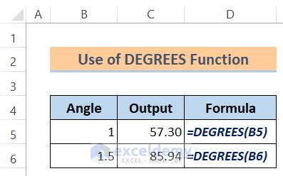
11. The DEGREES Function
- Function Objective:
The DEGREES function is applied to convert radians into degrees.
- Syntax:
=DEGREES(angle)
- Arguments Explanation:
| Argument | Required/Optional | Explanation |
|---|---|---|
| angle | Required | The angle in radians that we’ll convert. |
- Return Parameter:
Converts radians into degrees.
Use of DEGREES Function:
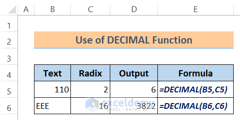
12. The DECIMAL Function
- Function Objective:
The DECIMAL function is used to convert a text representation of a number in a given base into a decimal number.
- Syntax:
=DECIMAL(text, radix)
- Arguments Explanation:
| Argument | Required/Optional | Explanation |
|---|---|---|
| text | Required | The text representation of the number that we want to convert. The length of the text must be less than or equal to 255 characters. |
| radix | Required | The base of the supplied number (An integer). |
- Return Parameter:
Converts a text representation of a number in a given base into a decimal number.
Use of DECIMAL Function:
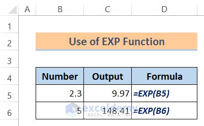
13. The EXP Function
- Function Objective:
The EXP function is used to return e raised to the power of number. The constant e equals 2.71828182845904 which is the base of the natural logarithm.
- Syntax:
=EXP(number)
- Arguments Explanation:
| Argument | Required/Optional | Explanation |
|---|---|---|
| number | Required | The exponent applied to the base e. |
- Return Parameter:
Returns e raised to the power of number.
Use of EXP Function:
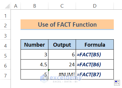
14. The FACT Function
- Function Objective:
The FACT function is applied to return the factorial of a number.
- Syntax:
=FACT(number)
- Arguments Explanation:
| Argument | Required/Optional | Explanation |
|---|---|---|
| number | Required | The nonnegative number for which we want the factorial. If the number is not an integer then it will be truncated. |
- Return Parameter:
The factorial of a number.
Use of FACT Function:
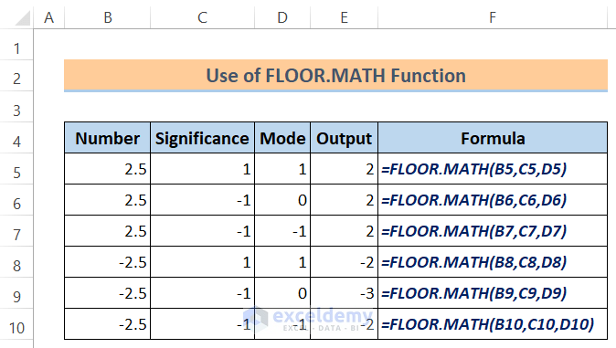
15. The FLOOR.MATH/FLOOR Function
- Function Objective:
The FLOOR.MATH function is applied to round a number down to the nearest integer or to the nearest multiple of significance.
- Syntax:
=FLOOR.MATH(number, significance, mode)
- Arguments Explanation:
| Argument | Required/Optional | Explanation |
|---|---|---|
| number | Required | The number is to be rounded down. |
| significance | Optional | The multiple to which we want to round. |
| mode | Optional | The direction for rounding negative numbers (toward or away from 0). |
- Return Parameter:
Rounds a number down to the nearest integer or to the nearest multiple of significance.
Use of FLOOR.MATH/FLOOR Function:
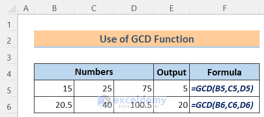
16. The GCD Function
- Function Objective:
The GCD function is applied to return the greatest common divisor of two or more integers. The greatest common divisor is the largest integer that divides both number1 and number2 without a remainder.
- Syntax:
=GCD(number1, [number2] …)
- Arguments Explanation:
| Argument | Required/Optional | Explanation |
|---|---|---|
| number1 | Required | Values from 1 to 255. If any value is not an integer then it will be truncated. |
| number2 | Optional | Values from 1 to 255. If any value is not an integer then it will be truncated. |
- Return Parameter:
The greatest common divisor of two or more integers.
Use of GCD Function:
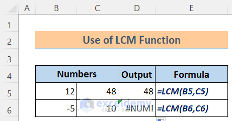
17. The LCM Function
- Function Objective:
The LCM function is used to return the smallest common multiplex of integers. The smallest common multiple is the least non-negative integer that is a multiplex of integer arguments number1, number2, and so on.
- Syntax:
=LCM(number1, [number2] …)
- Arguments Explanation:
| Argument | Required/Optional | Explanation |
|---|---|---|
| number1 | Required | Values from 1 to 255 for which we want the least common multiple. If a value is not an integer then it will be truncated. |
| number2 | Optional | Values from 1 to 255 for which we want the least common multiple. If a value is not an integer then it will be truncated. |
- Return Parameter:
The least common multiple of integers.
Use of LCM Function:
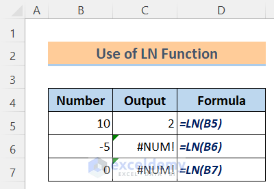
18. The LN Function
- Function Objective:
The LN function is used to return the natural logarithm of a number. Natural logarithms are based on the constant e (2.71828182845904).
- Syntax:
=LN(number)
- Arguments Explanation:
| Argument | Required/Optional | Explanation |
|---|---|---|
| number | Required | A positive real number for which we want the natural logarithm. |
- Return Parameter:
The natural logarithm of a number.
Use of LN Function:
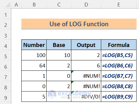
19. The LOG Function
- Function Objective:
The LOG function returns the logarithm of a number to the specified base.
- Syntax:
=LOG(number, [base])
- Arguments Explanation:
| Argument | Required/Optional | Explanation |
|---|---|---|
| number | Required | A positive real number for which we want the logarithm. |
| base | Optional | The base of the logarithm but If the base is omitted then it is assumed to be 10. |
- Return Parameter:
The logarithm of a number to the specified base.
Use of LOG Function:
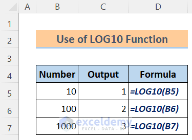
20. The LOG10 Function
- Function Objective:
The LOG10 function is applied to return the base-10 logarithm of a number.
- Syntax:
=LOG10(number)
- Arguments Explanation:
| Argument | Required/Optional | Explanation |
|---|---|---|
| number | Required | A positive real number for which we want the base10 logarithm. |
- Return Parameter:
The base-10 logarithm of a number.
Use of LOG10 Function:
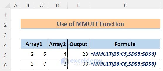
21. The MMULT Function
- Function Objective:
The MMULT function is used to return the matrix product of two arrays array1 and array2. The output is an array with the same number of rows as array1 and the same number of columns as array2.
- Syntax:
=MMULT (array1, array2)
- Arguments Explanation:
| Argument | Required/Optional | Explanation |
|---|---|---|
| array1 | Required | The first array that we want to multiply. |
| array2 | Required | The second array that we want to multiply. |
- Return Parameter:
The matrix product of two arrays array1 and array2.
Use of MMULT Function:
Read More: Top Excel Functions and Features for Management Consultants
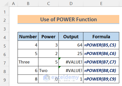
22. The POWER Function
- Function Objective:
The POWER function is used to return the result of a number raised to a power.
- Syntax:
=POWER(number, power)
- Arguments Explanation:
| Argument | Required/Optional | Explanation |
|---|---|---|
| number | Required | The base number can be any real number. |
| power | Required | The exponent to which the base number is raised. |
- Return Parameter:
The result of a number raised to a power.
Use of POWER Function:
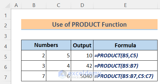
23. The PRODUCT Function
- Function Objective:
The PRODUCT function multiplies all the numbers given as arguments and returns the product.
For example, if cells B1 and B2 contain numbers, to multiply those two numbers together, we can use the formula:
= PRODUCT(B1, B2)
It’s the same as multiplying with the mathematical operator (*):
= B1 * B2
The PRODUCT Function is mainly useful when we need to multiply many cells together.
For example,
= PRODUCT(C1:C3, E1:E3)
is the same as
= C1 * C2 * C3 * E1 * E2 * E3
- Syntax:
=PRODUCT(number1, [number2] …)
- Arguments Explanation:
| Argument | Required/Optional | Explanation |
|---|---|---|
| number1 | Required | The first number or range that we want to multiply. |
| number2 | Optional | Additional numbers or ranges that we want to multiply, up to a maximum of 255 arguments. |
- Return Parameter:
Multiplies all the numbers given as arguments and returns the product.
Use of PRODUCT Function:
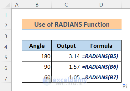
24. The RADIANS Function
- Function Objective:
The RADIANS function is applied to convert degrees to radians. The conversion is calculated by the formula:
180 degrees = π radians
Where π is the mathematical constant, Pi = 3.1416
- Syntax:
=RADIANS(angle)
- Arguments Explanation:
| Argument | Required/Optional | Explanation |
|---|---|---|
| angle | Required | An angle (in degrees) that we want to convert. |
- Return Parameter:
Converts degrees to radians.
Use of RADIANS Function:
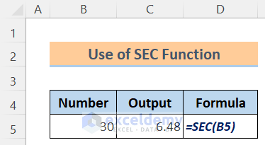
25. The SEC Function
- Function Objective:
The SEC function is used to return the secant of an angle.
- Syntax:
=SEC(number)
- Arguments Explanation:
| Argument | Required/Optional | Explanation |
|---|---|---|
| number | Required | The angle (in radians) for which we want the secant. |
- Return Parameter:
Returns the secant of an angle.
Use of SEC Function:
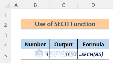
26. The SECH Function
- Function Objective:
The SECH function is applied to return the hyperbolic secant of an angle. The hyperbolic secant is the reciprocal of the hyperbolic cosine.
- Syntax:
=SECH(number)
- Arguments Explanation:
| Argument | Required/Optional | Explanation |
|---|---|---|
| number | Required | The number is the angle (in radians) for which we want the hyperbolic secant. |
- Return Parameter:
The hyperbolic secant of an angle.
Use of SECH Function:
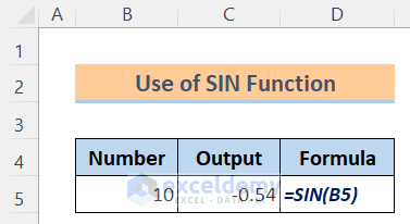
27. The SIN Function
- Function Objective:
The SIN function is used to return the sine of a given angle.
- Syntax:
=SIN(number)
- Arguments Explanation:
| Argument | Required/Optional | Explanation |
|---|---|---|
| number | Required | The angle (in radians) for which we want the sine. |
- Return Parameter:
The sine of the given angle.
Use of SIN Function:
28. The SINH Function
- Function Objective:
The SINH function is applied to return the hyperbolic sine of a number.
- Syntax:
=SINH(number)
- Arguments Explanation:
| Argument | Required/Optional | Explanation |
|---|---|---|
| number | Required | Any real number. |
- Return Parameter:
The hyperbolic sine of a number.
Use of SINH Function:

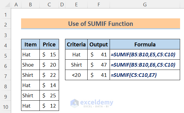
29. The SUMIF Function
- Function Objective:
The SUMIF function is used to sum the values in a range that meet the criteria that we specify.
- Syntax:
=SUMIF(range, criteria, [sum_range])
- Arguments Explanation:
| Argument | Required/Optional | Explanation |
|---|---|---|
| range | Required | The range of cells that we want to determine by criteria. The range of cells must be numbers or names, arrays or references that contain numbers. Blank and text values will be ignored. |
| criteria | Required | The criteria must be a number, expression, cell reference, text, or a function that defines which cells will be added. Any text criteria or any criteria that include logical or mathematical symbols must be enclosed in double quotation marks (“). Double quotation marks are not required for numeric criteria. |
| sum_range | Optional | The actual cells to add if we want to add cells other than those specified in the range argument. If sum_range is omitted then Excel will add the cells that are specified in the range. |
- Return Parameter:
The cells are specified by the given criteria.
Use of SUMIF Function:
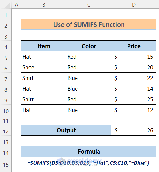
30. The SUMIFS Function
- Function Objective:
The SUMIFS function is applied to add all of its arguments that satisfy multiple criteria.
- Syntax:
=SUMIFS(sum_range, criteria_range1, criteria1, [criteria_range2, criteria2] …)
- Arguments Explanation:
| Argument | Required/Optional | Explanation |
|---|---|---|
| sum_range | Required | The range of cells to sum. |
| criteria_range1 | Required | The range that will be tested is based on Criteria1. Criteria_range1 and Criteria1 together search for specific criteria. If items in the range are found, the function adds the respective values. |
| criteria1 | Required | The criteria that are used to define which cells in Criteria_range1 will be added. |
| criteria_range2, criteria2, … | Optional | Other ranges and their related criteria. Maximum 127 range/criteria pairs can be entered. |
- Return Parameter:
The cells are specified by multiple criteria.
Use of SUMIFS Function:
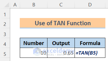
31. The TAN Function
- Function Objective:
The TAN function is applied to return the tangent of the given angle.
- Syntax:
=TAN(number)
- Arguments Explanation:
| Argument | Required/Optional | Explanation |
|---|---|---|
| number | Required | A real number as an angle. |
- Return Parameter:
The tangent of a number.
Use of TAN Function:
32. The TANH Function
- Function Objective:
The TANH function is used to return the hyperbolic tangent of a number.
- Syntax:
=TANH(number)
- Arguments Explanation:
| Argument | Required/Optional | Explanation |
|---|---|---|
| number | Required | A real number. |
- Return Parameter:
Returns the hyperbolic tangent of a number.
Use of TANH Function: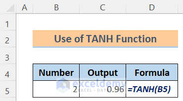
Read More: Compatibility Function in Excel
More Math and Trig Functions
33. The ACOS Function
- Function Objective:
The ACOS function is applied to return the arccosine or inverse cosine of a number. The arccosine is the angle whose cosine is a number. The returned angle is given in radians between 0 and π.
- Syntax:
=ACOS(number)
- Arguments Explanation:
| Argument | Required/Optional | Explanation |
|---|---|---|
| number | Required | The cosine of the angle we want must be from -1 to 1. |
- Return Parameter:
The arccosine of a number.
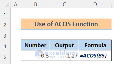
Use of ACOS Function:
34. The ACOSH Function
- Function Objective:
The ACOSH function is used to return the inverse hyperbolic cosine of a number. The inverse hyperbolic cosine is the value whose hyperbolic cosine is the number. So:
ACOSH (COSH (number)) = number
- Syntax:
=ACOSH(number)
- Arguments Explanation:
| Argument | Required/Optional | Explanation |
|---|---|---|
| number | Required | A real number equal to or greater than 1. |
- Return Parameter:
The inverse hyperbolic cosine of a number.
Use of ACOSH Function:

35. The ACOT Function
- Function Objective:
The ACOT function is applied to return the principal value of the arccotangent or inverse cotangent of a number as an angle, in radians, between 0 and π.
- Syntax:
=ACOT(number)
- Arguments Explanation:
| Argument | Required/Optional | Explanation |
|---|---|---|
| number | Required | The number is the cotangent of the angle we want which must be a real number. |
- Return Parameter:
The arccotangent of a number.
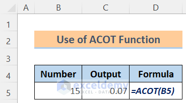
Use of ACOT Function:
36. The ACOTH Function
- Function Objective:
The ACOTH function is applied to return the inverse hyperbolic cotangent of a number.
- Syntax:
=ACOTH(number)
- Arguments Explanation:
| Argument | Required/Optional | Explanation |
|---|---|---|
| number | Required | The absolute value of a number must be less than -1 or greater than +1. |
- Return Parameter:
The hyperbolic arccotangent of a number.
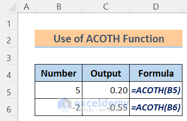
Use of ACOTH Function:
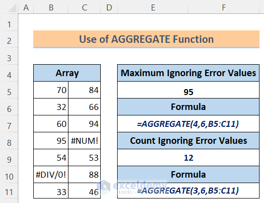
37. The AGGREGATE Function
- Function Objective:
The AGGREGATE function is used to apply various aggregate functions to a chart or database with the scope to avoid hidden rows as well as error values. It has two different formats −
- Reference Format
- Array Format
Reference Format
- Syntax:
=AGGREGATE(function_num, options, ref1, [ref2] …)
- Arguments Explanation:
| Argument | Required/Optional | Explanation |
|---|---|---|
| function_num | Required | A number 1 to 19 specifies which function to use. See the function_num table given below for the functions. |
| options | Required | A number, between 0 and 7, determines which values to be ignored in the calculation of the function. See the options table given below for the values. |
| ref1 | Required | The first argument(numeric) for the functions that accept multiplex numeric arguments for which we need the aggregate value. |
| [ref2] … | Optional | Numeric arguments (2 to 253) for which we need the aggregate value. |
- Return Parameter:
An aggregate in a list or database.
Array Format
- Syntax:
=AGGREGATE(function_num, options, array, [k])
- Arguments Explanation:
| Argument | Required/Optional | Explanation |
|---|---|---|
| function_num | Required | A number from 1 to 19 specifies which function to use. See the function_num table given below for the functions. |
| options | Required | A number, between 0 and 7, determines which values to be ignored in the calculation of the function. See the options table given below for the values. |
| array | Required | It can be an array, can be an array formula, or can be a reference to a group of cells for which we need the aggregate value. |
| k | Optional | An integer denotes the position in the array for functions that require this additional argument. Required for the ‘Large’, ‘Small’, ‘Percentile’ and ‘Quartile’ functions. See the argument k table given below. |
- Return Parameter:
An aggregate in a list or database.
Function_num Table:
| Function_num | Function |
|---|---|
| 1 | AVERAGE |
| 2 | COUNT |
| 3 | COUNTA |
| 4 | MAX |
| 5 | MIN |
| 6 | PRODUCT |
| 7 | STDEV.S |
| 8 | STDEV.P |
| 9 | SUM |
| 10 | VAR.S |
| 11 | VAR.P |
| 12 | MEDIAN |
| 13 | MODE.SNGL |
| 14 | LARGE |
| 15 | SMALL |
| 16 | PERCENTILE.INC |
| 17 | QUARTILE.INC |
| 18 | PERCENTILE.EXC |
| 19 | QUARTILE.EXC |
Argument [k] Table:
| Function | Meaning of k |
|---|---|
| Large | Returns the kth largest value. |
| Small | Returns the kth smallest value. |
| Percentile.Inc, Percentile.Exc | Returns the kth percentile. |
| Quartile.Inc, Quartile.Exc | Return the kth quartile. |
Use of AGGREGATE Function:
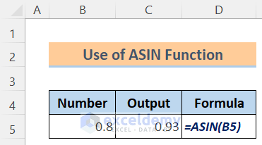
38. The ASIN Function
- Function Objective:
The ASIN function is applied to return the arcsine or inverse sine of a given number, and returns an angle in radians, between -π/2 and π/2.
- Syntax:
=ASIN(number)
- Arguments Explanation:
| Argument | Required/Optional | Explanation |
|---|---|---|
| number | Required | The sine of the angle we want must be from -1 to 1. |
- Return Parameter:
Returns the arcsine of a number.
Use of ASIN Function:
39. The ASINH Function
- Function Objective:
The ASINH function is used to return the inverse hyperbolic sine of a number. The inverse hyperbolic sine is the value whose hyperbolic sine is number:
ASINH (SINH (number)) = number
- Syntax:
=ASINH(number)
- Arguments Explanation:
| Argument | Required/Optional | Explanation |
|---|---|---|
| number | Required | A real number. |
- Return Parameter:
The inverse hyperbolic sine of a number.
Use of ASINH Function:

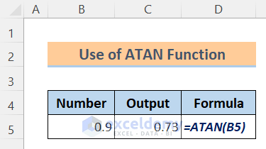
40. The ATAN Function
- Function Objective:
The ATAN function is applied to return the arctangent or inverse tangent of a number. The returned angle is given in radians between -π/2 and +π/2. The arctangent is the angle whose tangent is the number.
- Syntax:
=ATAN(number)
- Arguments Explanation:
| Argument | Required/Optional | Explanation |
|---|---|---|
| number | Required | The tangent of the angle we want. |
- Return Parameter:
The arctangent of a number.
Use of ATAN Function:
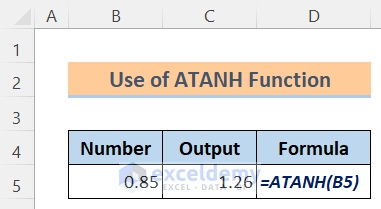
41. The ATANH Function
- Function Objective:
The ATANH function is used to return the inverse hyperbolic tangent of a number. The inverse hyperbolic tangent is the value whose hyperbolic tangent is the number. So:
ATANH(TANH (number)) = number
- Syntax:
=ATANH(number)
- Arguments Explanation:
| Argument | Required/Optional | Explanation |
|---|---|---|
| number | Required | A real number between (but not equal to) 1 and -1. |
- Return Parameter:
The inverse hyperbolic tangent of a number.
Use of ATANH Function:
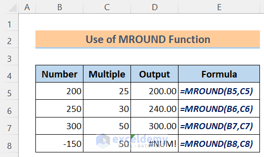
42. The MROUND Function
- Function Objective:
The MROUND function is used to return a number rounded to the desired multiple. MROUND function is one of fifteen rounding functions in Excel.
- Syntax:
=MROUND(number, multiple)
- Arguments Explanation:
| Argument | Required/Optional | Explanation |
|---|---|---|
| number | Required | The value to round. |
| multiple | Required | The multiple to which we want to round number. |
- Return Parameter:
A number rounded to the desired multiple.
Use of MROUND Function:
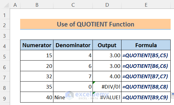
43. The QUOTIENT Function
- Function Objective:
The QUOTIENT function is applied to return the integer portion of a division. Apply this function when you want to discard the remainder of a division.
- Syntax:
=QUOTIENT(numerator, denominator)
- Arguments Explanation:
| Argument | Required/Optional | Explanation |
|---|---|---|
| numerator | Required | The dividend. |
| denominator | Required | The divisor. |
- Return Parameter:
The integer portion of a division.
Use of QUOTIENT Function:
44. The ROUND Function
- Function Objective:
The ROUND function is used to round a number to a specified number of digits. ROUND is one of the Excel Rounding Functions.
- Syntax:
=ROUND(number, num_digits)
- Arguments Explanation:
| Argument | Required/Optional | Explanation |
|---|---|---|
| number | Required | The number that you want to round. |
| num_digits | Required | The number of digits to which you want to round the number argument. |
- Return Parameter:
Rounds a number to a specified number of digits.
Use of ROUND Function:

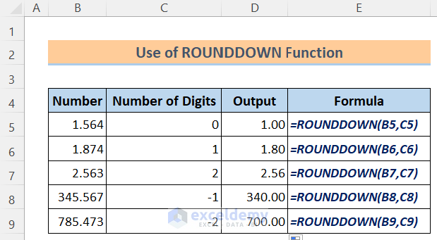
45. The ROUNDDOWN Function
- Function Objective:
The ROUNDDOWN function is used to round a number down, toward zero. ROUNDDOWN is one of the Excel Rounding Functions.
- Syntax:
=ROUNDDOWN(number, num_digits)
- Arguments Explanation:
| Argument | Required/Optional | Explanation |
|---|---|---|
| number | Required | A real number that we want to be rounded down. |
| num_digits | Required | The number of digits to which we want to round number. |
- Return Parameter:
Rounds a number down, toward 0.
Use of ROUNDDOWN Function:
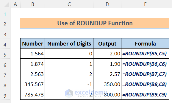
46. The ROUNDUP Function
- Function Objective:
The ROUNDUP function is applied to round a number up, away from 0 (zero). ROUNDUP is one of the Excel Rounding Functions.
- Syntax:
=ROUNDUP(number, num_digits)
- Arguments Explanation:
| Argument | Required/Optional | Explanation |
|---|---|---|
| number | Required | A real number that we want to be rounded up. |
| num_digits | Required | The number of digits to which we want to round number. |
- Return Parameter:
Rounds a number up, away from 0.
Use of ROUNDUP Function:
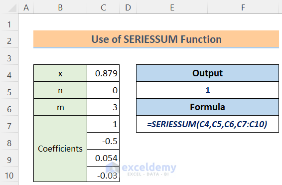
47. The SERIESSUM Function
- Function Objective:
The SERIESSUM function is applied to return the sum of a power series. It can approximate many functions by a power series expansion.
- Syntax:
=SERIESSUM(x, n, m, coefficients)
- Arguments Explanation:
| Argument | Required/Optional | Explanation |
|---|---|---|
| x | Required | An input value to the power series. |
| n | Required | The initial power to which we want to raise x. |
| m | Required | The step by which to increase n for each term in the series. |
| coefficients | Required | A set of coefficients by which we multiply every successive power of x, and the number of values in coefficients determines the number of terms in the power series. |
- Return Parameter:
The sum of a power series is based on the formula.
Use of SERIESSUM Function:
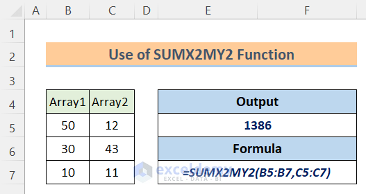
48. The SUMX2MY2 Function
- Function Objective:
The SUMX2MY2 function is applied to return the sum of the difference of squares of respective values in two arrays.
- Syntax:
=SUMX2MY2(array_x, array_y)
- Arguments Explanation:
| Argument | Required/Optional | Explanation |
|---|---|---|
| array_x | Required | The first array/range of values. |
| array_y | Required | The second array/range of values. |
- Return Parameter:
The sum of the difference of squares of corresponding values in two arrays.
Use of SUMX2MY2 Function:
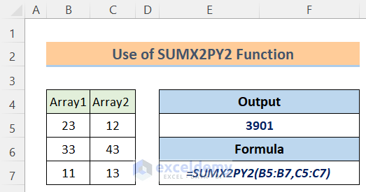
49. The SUMX2PY2 Function
- Function Objective:
The SUMX2PY2 function is used to return the sum of squares of corresponding values in two arrays.
- Syntax:
=SUMX2PY2(array_x, array_y)
- Arguments Explanation:
| Argument | Required/Optional | Explanation |
|---|---|---|
| array_x | Required | The first array/range of values. |
| array_y | Required | The second array/range of values. |
- Return Parameter:
The sum of squares of corresponding values in selected two arrays.
Use of SUMX2PY2 Function:
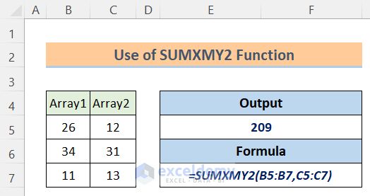
50. The SUMXMY2 Function
- Function Objective:
The SUMXMY2 function is applied to return the sum of squares of differences of corresponding values in two arrays.
- Syntax:
=SUMXMY2(array_x, array_y)
- Arguments Explanation:
| Argument | Required/Optional | Explanation |
|---|---|---|
| array_x | Required | The first array/range of values. |
| array_y | Required | The second array/range of values. |
- Return Parameter:
The sum of squares of differences of corresponding values in selected two arrays.
Use of SUMXMY2 Function:
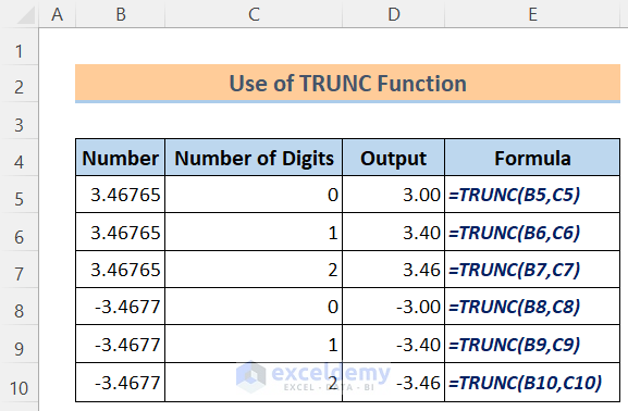
51. The TRUNC Function
- Function Objective:
The TRUNC function is applied to truncate a number to an integer by removing the fractional part of the number.
- Syntax:
=TRUNC(number, [num_digits])
- Arguments Explanation:
| Argument | Required/Optional | Explanation |
|---|---|---|
| number | Required | The number we want to truncate. |
| num_digits | Optional | A number that specifies the precision of the truncation. The default value for num_digits is 0. |
- Return Parameter:
Truncates a number.
Use of TRUNC Function:
Download Practice Workbook
Knowledge Hub
<< Go Back to Excel Function Categories | Excel Functions | Learn Excel
Get FREE Advanced Excel Exercises with Solutions!
