How to Use TAN Function in Excel (6 Examples)

The TAN function is in the Trigonometry Functions list under the Math and Trig Functions category that calculates the slope of a tangent of an angle of any triangle. We have other trigonometric functions available in Excel. In this article, we will discuss the use of the Excel TAN Function.

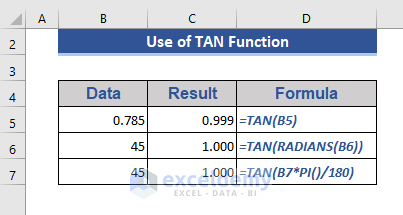
From the above image, you get a brief idea about the use of the TAN function in Excel.

TAN Function in Excel: Syntax

Function Objective:

The objective of this function is to get the tangent of an angle.

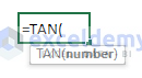
Syntax:

=TAN(number)

Argument:

Returns:

The return will be a tangent value.

Available in:

Excel for Microsoft 365, Microsoft 365 for Mac, Excel for the web Excel 2021, Excel 2021 for Mac, Excel 2019, Excel 2019 for Mac, Excel 2016, Excel 2016 for Mac, Excel 2013, Excel 2010, Excel 2007, Excel for Mac 2011, Excel Starter 2010.

Note:

Our arguments must be in radians. If the argument is in the degree we must multiply it by Pi()/180 or use the RADIANS function.

What is the Tangent Ratio in Trigonometry?

The tangent or tan ratio comes from the tangent line of the trigonometry named Tangent. Sine and Cosine are also some trigonometric ratios. The tan ratio is based on a right-angle triangle. It is defined as the ratio of the opposite arm and the adjacent arm of the right angle.

So, the tangent angle can be expressed in the following way.

Tangent is also expressed as the ratio of Sine and Cosine.

Here, we will show some examples of how to use the TAN function in Excel.

1. Using the TAN Function with Radians

In this example, we will show how to use the TAN function with radians. Here, we have taken a data set that consists of radian values.

We can use these radians directly in the TAN function. Now, follow the steps below.

Step 1:

• Click on Cell C5.
• Now type the following formula-

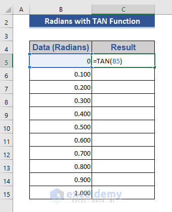
Step 2:

• Now, press Enter.

We get the slope of a tangent at 0 radians.

Step 3:

• Pull the Fill Handle icon all the way.

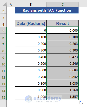
We get the tangent value of all the radians mentioned here.

2. Combining the TAN and PI Functions

Here we will use the PI function with the TAN function.

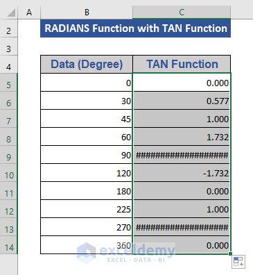
In our data set all the values are in degrees.

Step 1:

• We will multiply this data by PI()/180 to convert in radians and apply the TAN function with the formula:

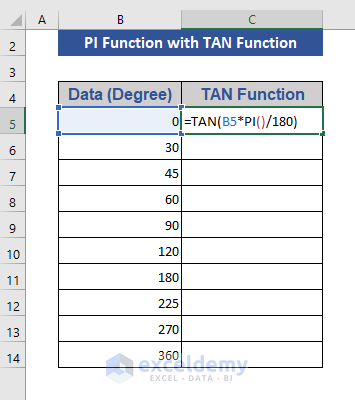
Step 2:

• Now, press the Enter.

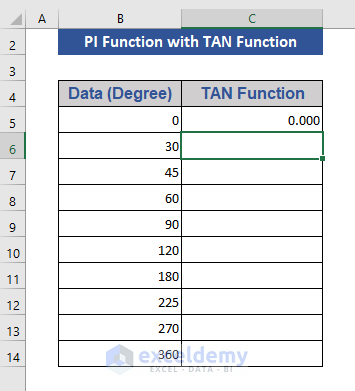
Step 3:

• Drag the pull Fill Handle icon to the last cell.

Here, we get the slope of the tangents against our input data.

Note:
###### refers that we get infinite values for tangents 90, 270 degrees.

3. Using TAN and RADIAN Functions in Excel

Here we will use the RADIANS function with the TAN function. The RADIANS function is used here as our data is in degree.

We will consider the below data for this example.

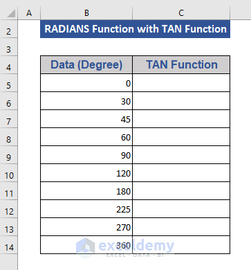
Here, we need to convert the degrees into radians.

Step 1:

• Go to Cell C5.

We will coincide the RADIANS function with the TAN function.

• Write the following formula:

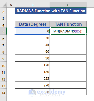
Step 2:

• Now, press Enter.

Step 3:

• Now, pull the Fill Handle icon towards the last cell.

We get the slope for the tangents for all the data taken as degrees.

Note:
###### indicates that we get infinite values for tangents 90, 270 degrees.

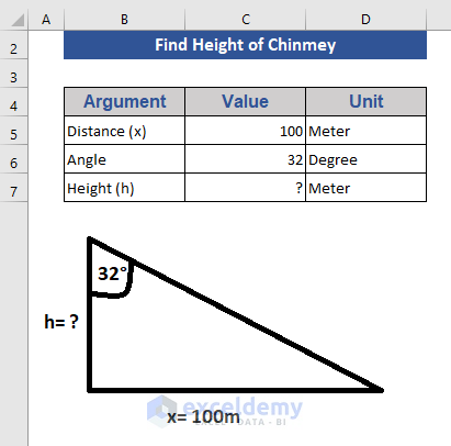
4. Calculating the Height of a Chimney Using the TAN Function in Excel

In this example, we will consider a chimney that can be from a distance of 100 m at an angle of 32°. We will find out the height of the chimney here.

We already know that,

Tangent angle = Opposite Side/Adjacent Side

Here, we have the data of a chimney below.

Step 1:

• Now, we will apply the below formula to find the height.

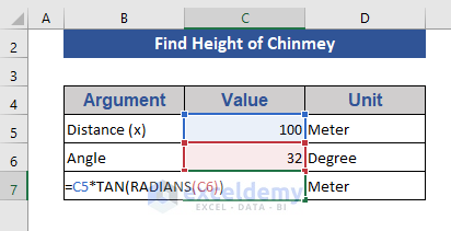
Here, we multiplied the perpendicular by the tangent angle.

Step 2:

• Finally, press Enter.

Here, we get the height of a chimney by applying the TAN function.

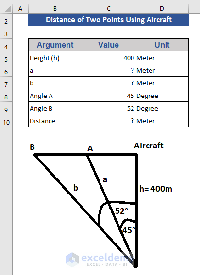
5. Finding the Distance of Two Points from an Aircraft Using the Excel TAN Function

This example is based on an aircraft.

We assume that an aircraft is flying at a height of 400 m. Now, two points A and B are in the direction of the aircraft with angles 45° and 52° respectively. Now, we find out the distance between A and B.

Data presentation of this example is below:

Step 1:

• Click on Cell C6.
• Enter the following formula-

Step 2:

• Then, press Enter.

Step 3:

• Apply the same formula by changing the corresponding argument at Cell C7.
• Then press Enter.

Step 4:

• Write the subtraction formula at Cell C10. The formula is:

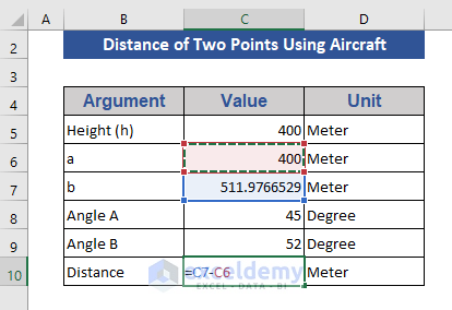
Step 5:

• Then, press Enter.

The above picture shows the distance between the two points.

6. Calculating the Area of a Trapezoid Using TAN Function in Excel

In this example, we will show how to find the length of the arms of the trapezoid.

We will consider the data in the following image for this example.

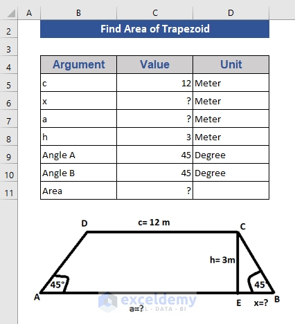
We will find the area of the trapezoid. That is-

Step 1:

• Go to Cell C6.
• Get the value of ‘a’ by applying the following formula-

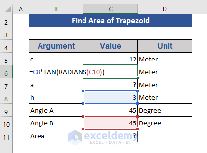
Step 2:

• Then, press Enter.

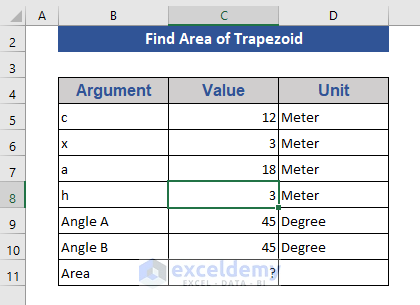
Step 3:

• Now, get the value of applying the following formula at Cell C7.

Step 4:

• Then press Enter.

Step 5:

• Now, we will find the area of the trapezium.
• Apply the following formula to Cell C11.

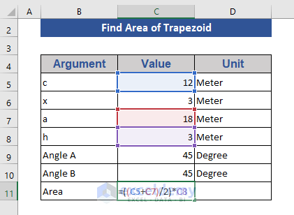
Step 6:

• Then press Enter.

This is the area of the trapezium.

Things to Remember

• The input data must be in radians format.
• If the input data is degree format. Then first convert to radians format and apply the TAN function.

Download Practice Workbook

Download the following practice workbook to exercise while you are reading this article.

Conclusion

In this article, we described how to use the TAN function in Excel. I hope this will satisfy your needs. Please give your suggestions and feedback in the comment box.