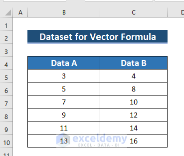
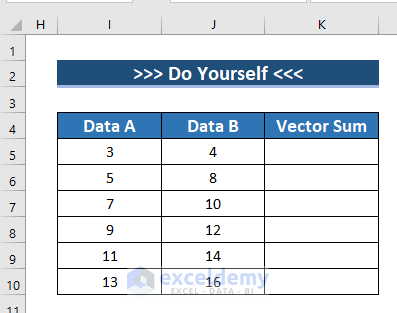
The following dataset showcases vector data: Data A and Data B.
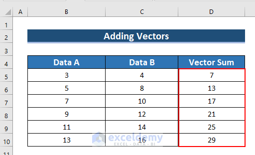
Example 1 – Using an Addition Formula to Sum Two Vector Data
Steps:
- Enter the following formula in D5.
=B5:B10+C5:C10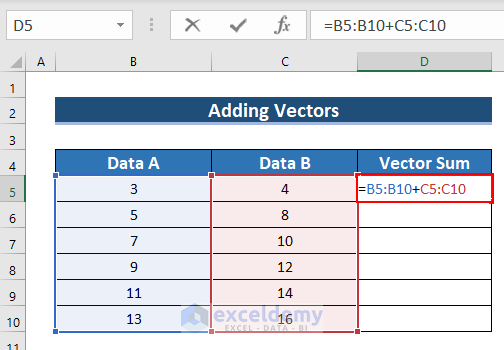
- Since this is an ARRAY formula press CTRL+SHIFT+ENTER. (For Excel 365, press ENTER.)
- See the result in D5:D10.
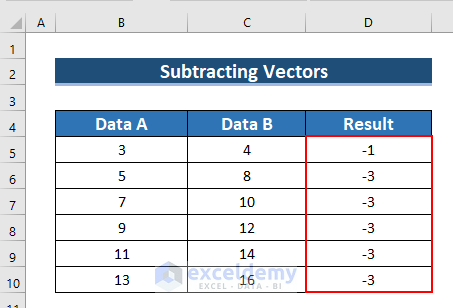
Example 2 – Use a Subtraction Formula to Deduct One Vector Data from Another
Steps:
- Enter the following formula in D5.
=B5:B10-C5:C10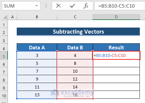
- Since this is an ARRAY formula press CTRL+SHIFT+ENTER. (For Excel 365, press ENTER.)
- See the result in D5:D10.
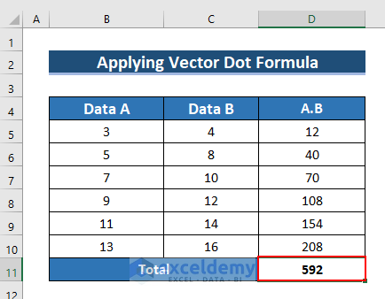
Example 3 – Using a Vector Dot Formula for Two Sets of Vector Data
3.1. Generic Formula
Steps:
- Enter the following formula in D5.
=C5*B5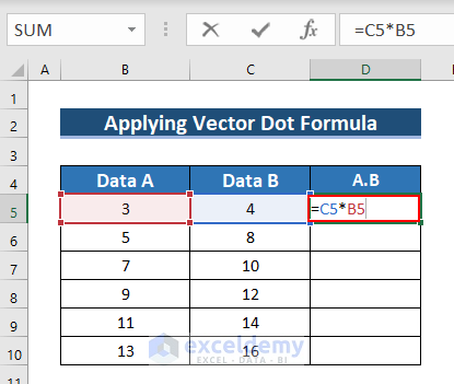
- Press ENTER.
- See the result in D5.
- Drag down the formula with the Fill Handle tool.
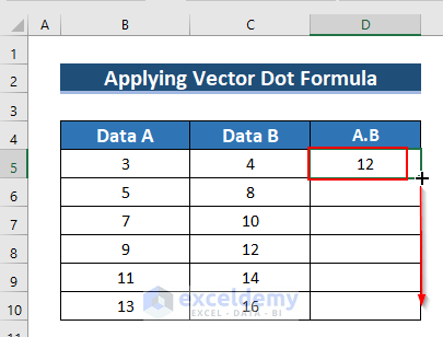
- This is the output.

- To find the sum of this multiplication: enter the following formula in D11.
=SUM(D5:D10)The SUM function sums the cell range.
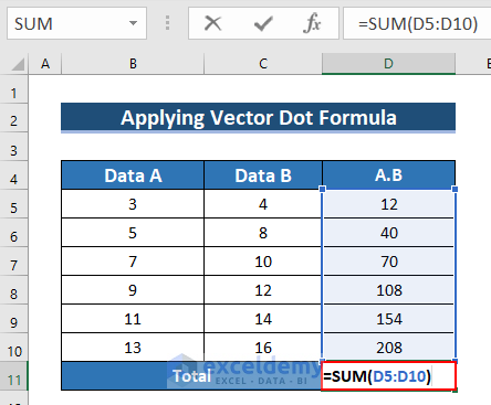
- Press ENTER.
- See the result in D11.
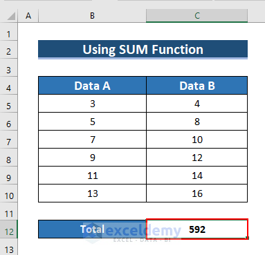
3.2. Applying the SUM Function
Steps:
- Enter the following formula in C12.
=SUM(B5:B10*C5:C10)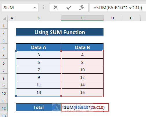
- Press CTRL+SHIFT+ENTER.
- See the result in C5:C10.
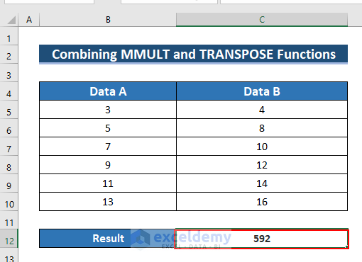
3.3. Combining the MMULT and the TRANSPOSE Functions
Steps:
- Enter the following formula in C12.
=MMULT(TRANSPOSE(B5:B10),(C5:C10))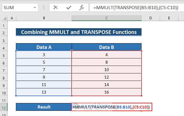
Formula Breakdown
- The MMULT function returns the matrix product of two cell ranges.
- The TRANSPOSE function modifies the orientation of the cell range.
- TRANSPOSE(B5:B10)→ becomes
- Output: {3,5,7,9,11,13}
- MMULT(TRANSPOSE(B5:B10),(C5:C10) → becomes
- MMULT({3,5,7,9,11,13}),(C5:C10))
- Output: 592
- MMULT({3,5,7,9,11,13}),(C5:C10))
- Press ENTER.
- See the result in C12.
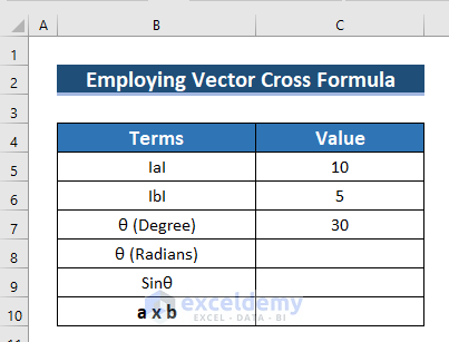
Example 4 – Using a Vector Cross Formula for Two Sets of Vector Data
The following dataset showcases the value of IaI (value of the first vector), IbI (value of the second vector), and the angle between them θ in degree.
- Convert the angle to Radians. and find the cross multiplication by using the formula a x b=IaI IbI Sinθ
Steps:
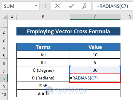
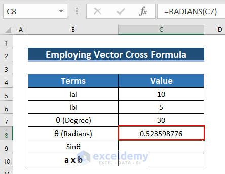
- Convert the Degree to Radians: Enter the following formula in C8.
=RADIANS(C7)The RADIANS function converts the degree into radians.
- Press ENTER.
- See the result in C8.
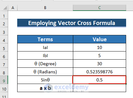
- To find the Sinθ, use the following formula in C9.
=SIN(C8)The SIN function converts the Radian angle into the sin angle.
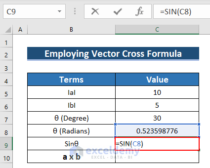
- Press ENTER.
- See the result in C9.
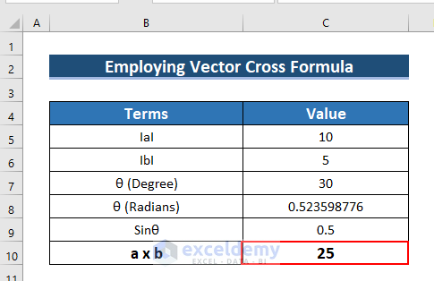
- To find the cross-product, enter the following formula in C10.
=C5*C6*C9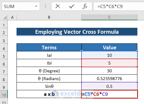
- Press ENTER.
- See the output in C10.
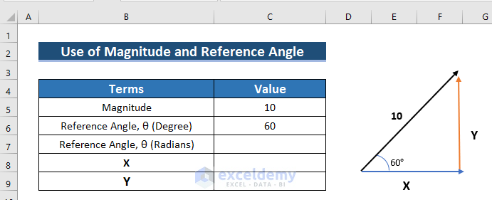
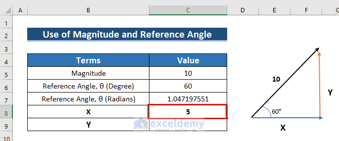
Example 5 – Using a Vector Formula to Find Two Components Using Magnitude and Reference Angle of This Vector
In the image below the magnitude of a vector is 10, and the direction is 60°. You want to find X and Y.
X = 10 Cosθ
Y=10 Sinθ
Data was inserted in the dataset.
Steps:
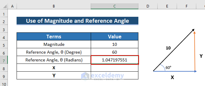
- Convert Degrees to Radians, using the following formula in C7.
=RADIANS(C6)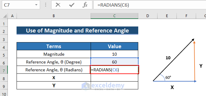
- Press ENTER.
- See the result in C8.
- To find X, enter the following formula in C8.
=C5*COS(C7)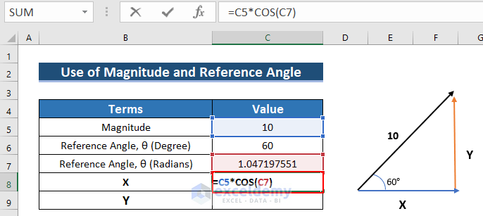
- Press ENTER.
See the result in C8.
- To find Y, enter the following formula in C9.
=C5*SIN(C7)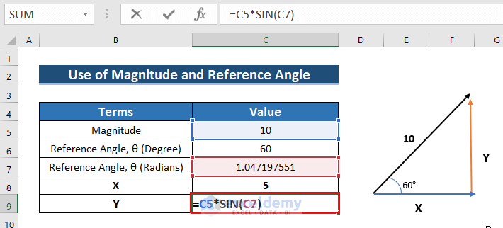
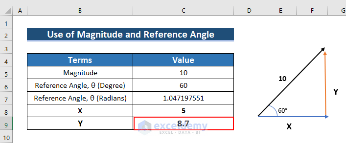
- See the outcome in C9.
This is the output.
Practice Section
Download the following Excel file and practice.
Download Practice Workbook
Download the Excel file and practice.
Vector Formula in Excel: Knowledge Hub
- How to Calculate Vector Multiplication in Excel
- How to Calculate Eigenvectors in Excel
- How to Calculate Eigenvalues and Eigenvectors in Excel
<< Go Back to | Excel for Math | Learn Excel
Get FREE Advanced Excel Exercises with Solutions!
