We may often need to use the Math & Trig functions in Excel for different calculating purposes. In this article, I’ll introduce you to one of them that is the FACT function in Excel.
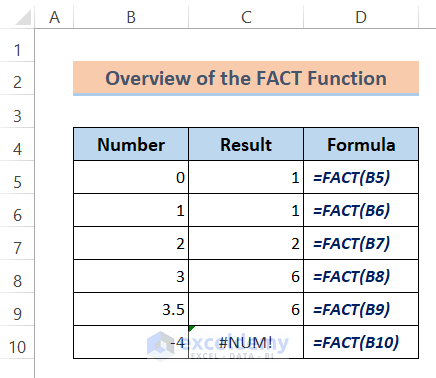
The above screenshot is an overview of the FACT function. This article will guide you with easy examples to use the application of the FACT function.
Introduction to the FACT Function

The FACT function is a mathematical operator categorized under the Math & Trig function which is used to return the factorial of a number. Factorial of a number (n) can be calculated using the following formula:
n!=1*2*3*……*(n-1)*n
So the factorial of 5 will be-
5!=5*4*3*2*1=120
That means the factorial of a number is the multiplication of all the numbers decreased by 1 starting from the number and ending to 1.
Purpose of the FACT Function:
The FACT function is used to get the factorial of a number.
Syntax:
=FACT(number)Arguments:
| Arguments | Required/Optional | Explanation |
|---|---|---|
| number | Required | The nonnegative number for which we want the factorial. If the number is not an integer then it is truncated. |
Returns:
The factorial of a number.
How to Use the Excel FACT Function: 2 Easy Examples
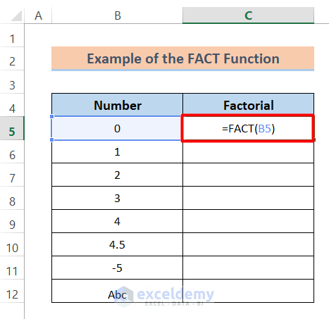
Let’s get introduced to our dataset first. I have used some integer, negative numbers, and non-numeric values in my dataset.

Example 1: Excel FACT Function in Worksheet
Now we’ll find the factorial of each value from the range B5:B12.
Steps:
⏩ Activate Cell C5.
⏩ Then type the following formula given below in it-
=FACT(B5)⏩ Later, press the Enter button for the output.
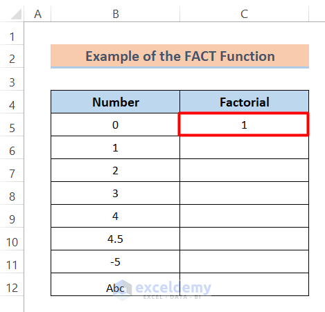
Then you will get the factorial for 0 is 1.
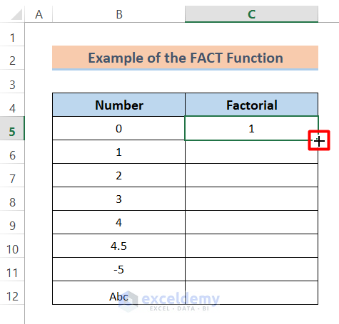
To get the factorials for the other values just drag the Fill Handle icon.
Now you get all the factorials for the numbers like the image below. Take a look at the output that there are two errors. The FACT function will return #NUM if the given number is less than 0. It will show #VALUE if it finds a non-numeric value. And if the given number is not an integer then it will truncate the decimal portion that’s why the factorials of 4 and 4.5 are the same.

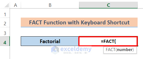
Example 2: FACT Function with Keyboard Shortcut
We can calculate the factorial of a number using the FACT function in a different way. Here, we’ll use a keyboard shortcut with the FACT function. Let’s see how to do it.
Steps:
⏩ Write the following formula in Cell C4–
=FACT(⏩ Then press Ctrl+A on your keyboard.
A dialog box will open up.
⏩ Type the number in the Number box.
⏩ Finally, just press OK.
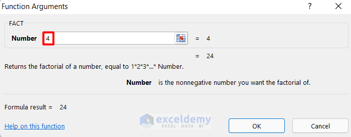
Then you will see that the factorial is calculated.

Read More: How to Calculate Factorial of Large Number in Excel
Download Practice Workbook
You can download the free Excel template from here and practice on your own.
Conclusion
I hope all of the methods described above will be good enough to use the FACT function in Excel. Feel free to ask any question in the comment section and please give me feedback.
FACT Function in Excel: Knowledge Hub
- How to Do Factorial in Excel
- How to Use FACTDOUBLE Function in Excel
- How to Calculate Factorial Using Excel VBA
<< Go Back to Excel Functions | Learn Excel
Get FREE Advanced Excel Exercises with Solutions!
