How to Draw Circle in Excel (4 Simple Methods)

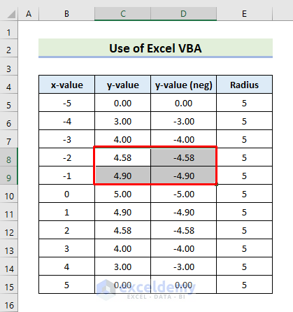
The sample dataset that represents circular components and values. We will use these number values to draw a circle in Excel.

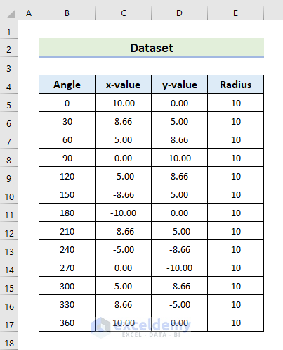
Method 1 – Enter Mathematical Equation to Plot a Circle in Excel

If we draw a circle and the center of the circle coincides with the origin of the (x,y) plane, the center is (0,0).  Here, at any point on the circle, if the coordinates are (x,y), then the relationship between x & y and the radius r is,

• Which is our Pythagorean theorem.

We can also write

We can this formula to draw a circle.

Steps:

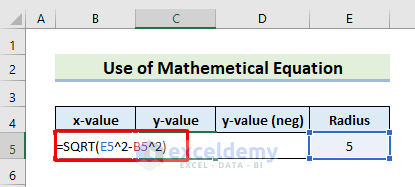
• Take -5 and 5 as the values of x and Radius.
• Enter the formula for the y-value in cell C5

• Hit Enter or the Tab key.

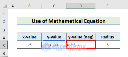
• The y values will only return a semi-circle. To draw a full circle, we also need -y values.
• To calculate -y values, in cell D5, enter:

• The -y values are returned in column D.

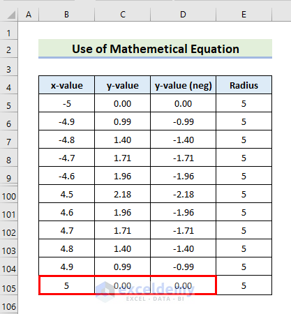
• Drag the formula cells down to row 105 to AutoFill the cells.
• The first values and last values will repeat as shown below.

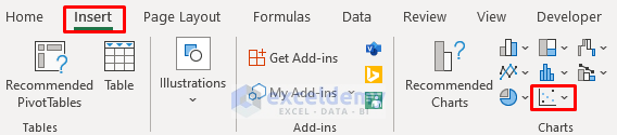
• Go to Insert and navigate to the Charts group.
• Select Insert Scatter (X, Y) or Bubble Chart option in the ribbon.

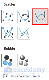
• A dropdown box will appear.
• Click the Scatter with Smooth Line option.

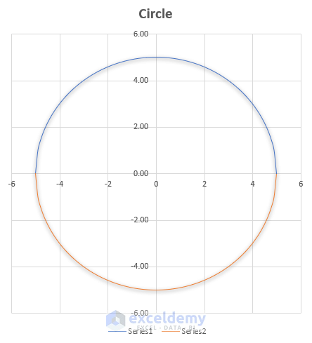
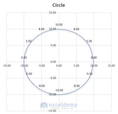
• This will create a circle.

Method 2 – Use SIN & COS Functions to Create a Circle in Excel

The SIN function takes in the angles in the corresponding radians and returns the sine angles while the COS function determines the cosine value of an angle after evaluating the angles to radians. We can use these functions to create a circle in our dataset.

Steps:

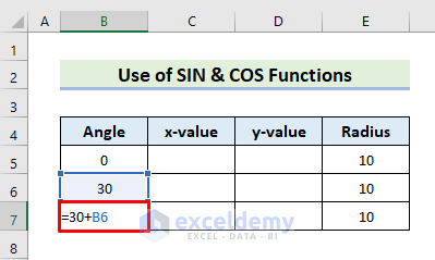
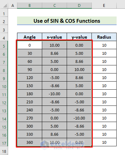
• Set the radius as 10 in column E.
• Input the angle values in column B.
• We need the angle after every 30 consecutive numbers, as shown in the following formula:

• AutoFill the table by dragging the cell down up to 360 value.

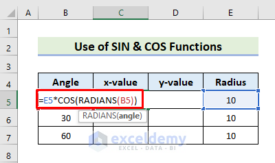
• Determine the x-value by using COS.
• In cell C5, enter the following formula:

• Press Enter to get the value.

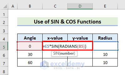
• Determine the value of y using the SIN function with the below formula.

• Hit Enter or Tab to obtain the y values.

• AutoFill the columns.
• Select the range B5:D17 to insert the values in a chart.

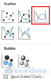
• Go to the Insert tab and click the Insert Scatter (X,Y) or Bubble Chart option in the Charts group.
• The Scatter dropdown box pops up.
• Click Scatter with Smooth Lines option.

• We get the desired circle in a chart.

Read More: How to Draw a Mohr Circle in Excel 

Method 3 – Draw a Circle Using Excel Shape Tool

Steps:

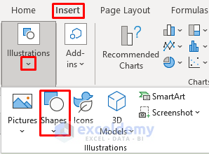
• Go to Insert > Illustrations > Shapes tab.

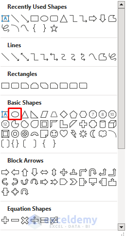
• The shape options box will appear.
• Go to Basic Shape and select the Oval option.

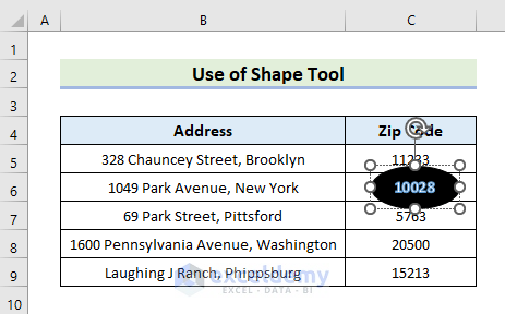
• The circle pops up in the dataset.
• You can drag the circle to highlight any cells as well.

Read More: How to Put a Circle Around a Number in Excel 

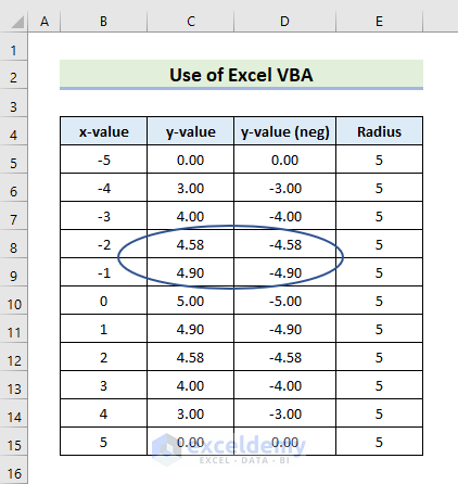
Method 4 – Make a Circle Using Excel VBA

Steps:

• Select the range C8:D9 to circle around multiple cells to group them together.

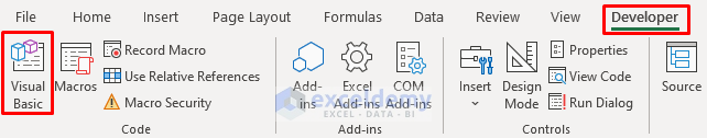
• Go to the Developer tab, and click Visual Basic.

• The Visual Basic window will pop up.
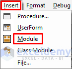
• Select Insert and then Module to create a module.

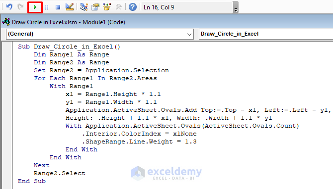
• Enter the following VBA code:

Sub Draw_Circle_in_Excel()
Dim Range1 As Range
Dim Range2 As Range
Set Range2 = Application.Selection
For Each Range1 In Range2.Areas
With Range1
x1 = Range1.Height * 1.1
y1 = Range1.Width * 1.1
Application.ActiveSheet.Ovals.Add Top:=.Top - x1, Left:=.Left - y1, _
Height:=.Height + 1.1 * x1, Width:=.Width + 1.1 * y1
With Application.ActiveSheet.Ovals(ActiveSheet.Ovals.Count)
.Interior.ColorIndex = xlNone
.ShapeRange.Line.Weight = 1.3
End With
End With
Next
Range2.Select
End Sub

• Press the green Run button to execute the code.

• The circles will appear in the dataset.
• Drag the circle to select any specific cells you wish.

Read More: How to Circle Something in Excel 

Download Practice Workbook

Download this practice workbook to exercise while you are reading this article.

Draw Circle in Excel: Knowledge Hub

• How to Circle Text in Excel 
• How to Create Concentric Circle Chart in Excel
• How to Draw a Circle in Excel with Specific Radius

<< Go Back to Learn Excel