Today, we will show how to draw a Mohr Circle in Excel. The Mohr’s Circle is a powerful engineering visualization tool. It is a sophisticated way to visualize the normal stress, shear stress and the relation between the two stresses acting on a stress element at any orientation. This is also very helpful in determining the shear and normal stress for a particular angle.
What Is Mohr Circle?
The Mohr’s Circle is a graphical representation of stresses in a plane. It outlines the normal and shear stresses acting on a stress element and also shows the relation of the stresses. By using the Mohr’s Circle, one can calculate the normal and shear stress on a plane quickly and effectively. One can also calculate the maximum shear and normal stresses on the plane from this circle.
How to Draw a Mohr Circle in Excel: Step-by-Step Procedure
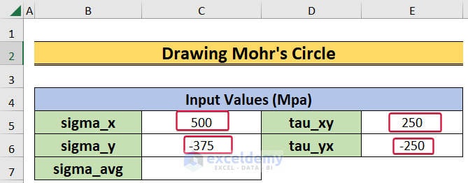
In this article, we will show a comprehensive step-by-step procedure of how to draw a Mohr’s Circle in Excel. We will use the Scatter Chart to plot the stress values and draw the circle. Here, we have a dataset of a stress element which has a normal stress of 500 Mpa in the X direction (sigma_x) and a normal stress of 375 Mpa in the Y direction (sigma_y). sigma_y is negative because it is a compressive stress. Finally, the stress element has a shear stress of 250 Mpa in the XY plane. We will use these datasets to draw the Mohr’s Circle.
Step 1: Calculating Average Normal Stress
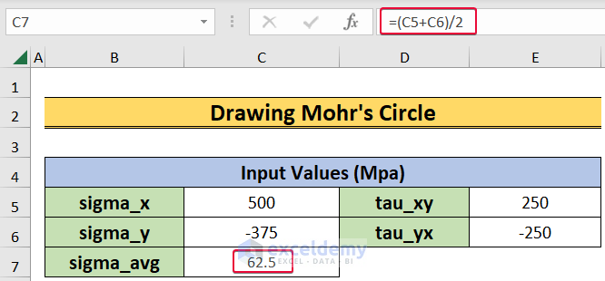
In this step, we will calculate the average normal stress on the element. This is the average of the normal stress in the X direction and that of in the Y direction.
- Firstly, choose the C7 cell and enter the following,
=(C5+C6)/2
- Then, hit Enter.
- As a result, we will have the average normal stress.
Read More: How to Circle Something in Excel
Step 2: Determining Radius
Here, we will calculate the radius of the Mohr’s Circle. We will use the normal stress in the X direction, the average normal stress and the shear stress to get the value. We will also use the SQRT function here.
- To begin with, choose the C9 cell and type,
=SQRT((C5-C7)^2+E5^2)
- Then, press Enter.
- As a result, we will get the radius of the circle.

Read More: How to Draw a Circle in Excel with Specific Radius
Step 3: Inserting Angles and Converting to Radians
In this instance, we will insert angles in degrees to draw the circle and convert them in radians to use them in formulas. We will add 360 degrees as a circle contains 360 degrees. We will also convert the degrees into radians by using the RADIANS function.
- At the beginning, choose the C12 cell and write zero degree.

- Next, type the following in the C13 cell,
=C12+1
- Press Enter.
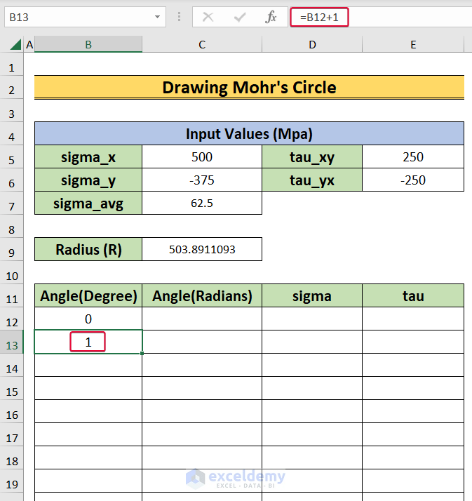
- As a result, we will get the degree.
- Now, lower the cursor down until we reach the 360-degree value.

- Thereafter, choose the C12 cell and insert,
=RADIANS(B12)
- Now, hit Enter.
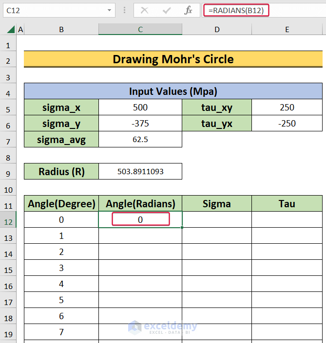
- As a result, we will get the radian value for zero degree.
- Next, move the cursor down to autofill.
Step 4: Calculating Normal Stress
In this step, we will calculate the normal stresses (Sigma) on the body for every orientation or in other words for 360 degrees. This calculation involves the COS function.
- At the start, choose the D12 cell and enter the following formula,
=$C$9*COS(C12)+$C$7
- Next, hit Enter.
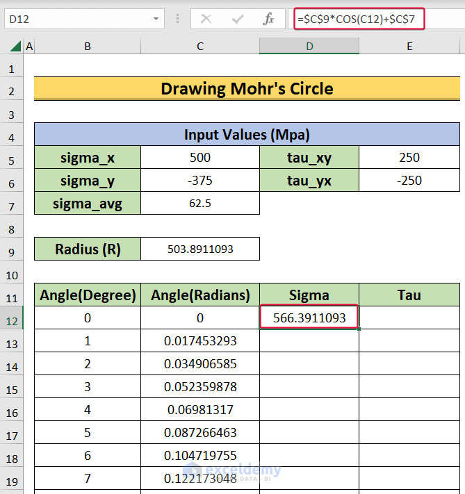
- Consequently, we will get the normal stress value for zero degree.
- Finally, move the cursor down to the D372 cell to autofill the values.
Step 5: Measuring Shear Stress
Next, we will measure the shear stress (tau) on the element. Shear stress is a stress that acts parallel to the surface. Here, we will use the SIN function.
- Firstly, click on the E12 cell and type,
=$C$9*SIN(C12)
- Now, press Enter.
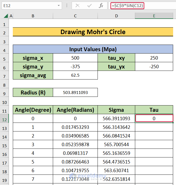
- As a result, we will have the shear stress for zero degree.
- Finally, slide the cursor down to the E372 cell to autofill.
Step 6: Drawing Mohr’s Circle
In this final method, we will draw the Mohr’s Circle. We will plot the data in a Scatter chart. We will create data series to draw the circle properly.
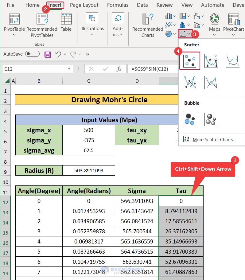
- Firstly, choose the E12 cell and press Ctrl+Shift+Down Arrow.
- Secondly, go to the Insert
- Thirdly, choose Insert Scatter (X,Y) or Bubble Chart from the Charts
- Finally, from the drop-down list, choose the Scatter Chart.
- As a result, a graph will be plotted.
- Now, right-click on the graph and choose Select Data.
- As a result, a prompt will appear on the screen.

- In the prompt, remove the existing data series by clicking

- Then, choose Add to add new data series.
- Consequently, the Edit Series prompt will appear.

- In the prompt, first, set the Series name to Mohr’s Circle.
- Secondly, select the D12:D372 range as the Series X values.
- Thirdly, choose the E12:E372 cell range and set it as Series Y values.
- Finally, choose OK.

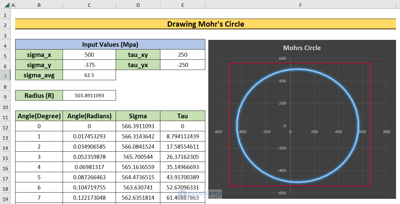
- Consequently, we will have the Mohr’s Circle for those stress values.
- You could format the graph to make it more eloquent.
This is how we will draw a Mohr Circle in Excel.
Read More: How to Put a Circle Around a Number in Excel
Download Practice Workbook
You can download the practice workbook here.
Conclusion
In this article, we have talked about how to draw a Mohr Circle in an exhaustive way. This will allow users to plot and visualize the Mohr’s Circle more effectively. If you have any questions regarding this essay, feel free to let us know in the comments.
Related Articles
<< Go Back to Circle in Excel | Learn Excel
Get FREE Advanced Excel Exercises with Solutions!
