How to Create Concentric Circle Chart in Excel (with Easy Steps)

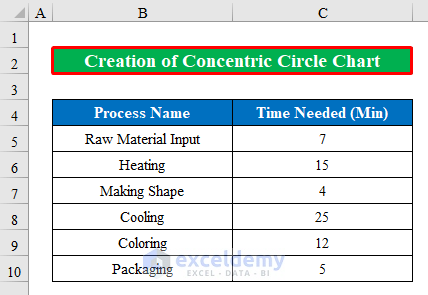
Step 1 – Creating the Dataset with the Proper information

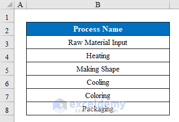
We have a list of processes in a company which we’ll chart.

• Insert the list in a column.

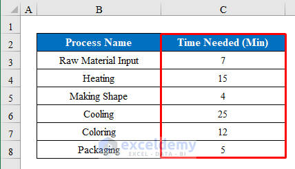
• Create another table and put the Time Needed for each process.

• Put a header at the top of the dataset.

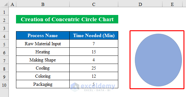
Step 2 – Inserting Oval Shapes for the Concentric Circle Chart

• Choose the Oval shape from the Shapes option.

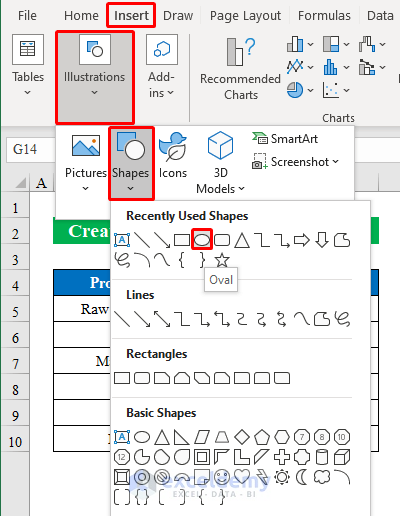
• Draw a shape inside the worksheet.

• Select the newly created shape and press Ctrl + C to copy.

• Press Ctrl + V to paste, and you will get another shape.

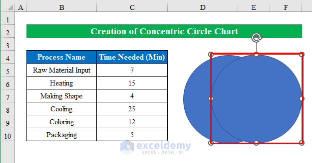
• Resize the new shape inside the previous one.

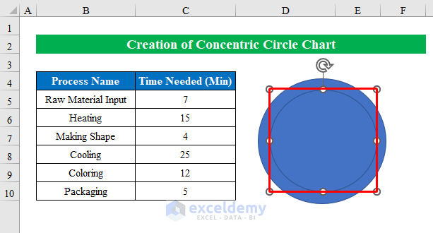
• Repeat to create multiple circles.

Read More: How to Draw a Circle in Excel with Specific Radius 

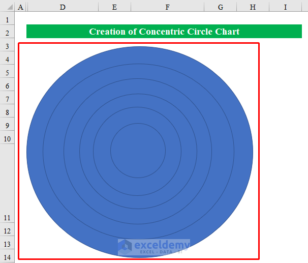
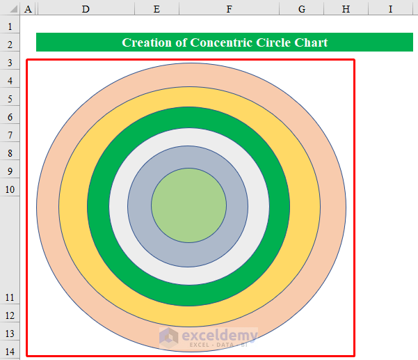
Step 3 – Coloring and Editing the Chart

• Choose a circle and select your desired color from the Home ribbon.

• Color other circles.

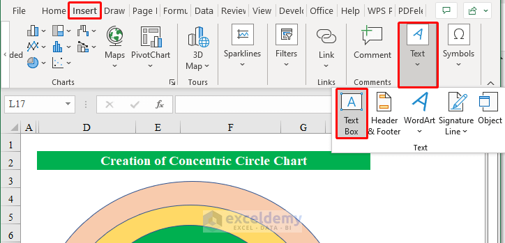
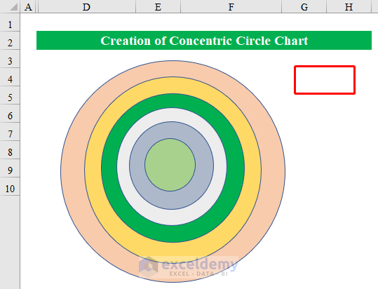
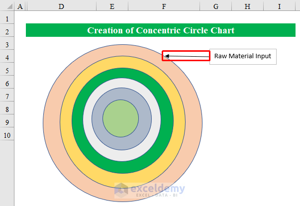
• Insert a Text Box from the Insert feature to name the processes.

• Draw the box inside the worksheet.

• Put your desired process names from the data table.

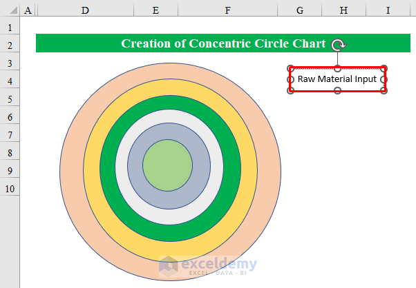
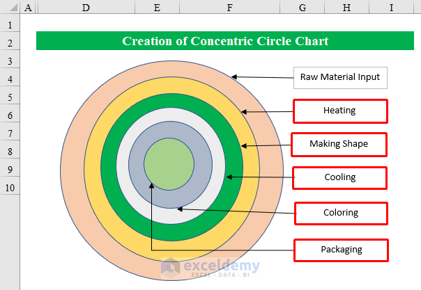
• Connect the text box and a circle with a LineArrow.

• Repeat to create text boxes for other processes and connect them with their circles.

Read More: How to Draw a Mohr Circle in Excel

Things to Remember

• You can also insert a StackedVenn chart from the SmartArt Graphic command.

Download the Practice Workbook

Related Articles

• How to Circle Something in Excel
• How to Circle Text in Excel
• How to Put a Circle Around a Number in Excel

<< Go Back to Circle in Excel | Learn Excel