This tutorial will demonstrate how to calculate quartile deviation in Excel. It is essential to use quartile deviation in almost every aspect of our lives. Quartiles are the most effective when we want to find the center of certain data. This shows us the variability of the values of certain datasets. We can use it in case of sales in the company, marks, etc. So, it is important to learn how to calculate quartile deviation in Excel.
How to Calculate Quartile Deviation in Excel: 4 Easy Methods
We’ll use a sample dataset overview as an example in Excel to understand easily. If you can calculate deviation in Excel, then you can easily calculate quartile deviation in Excel. Following the steps correctly may help you to learn how to calculate quartile deviation in Excel promptly. The methods are
1. Calculating Quartile Deviation for Linear Data
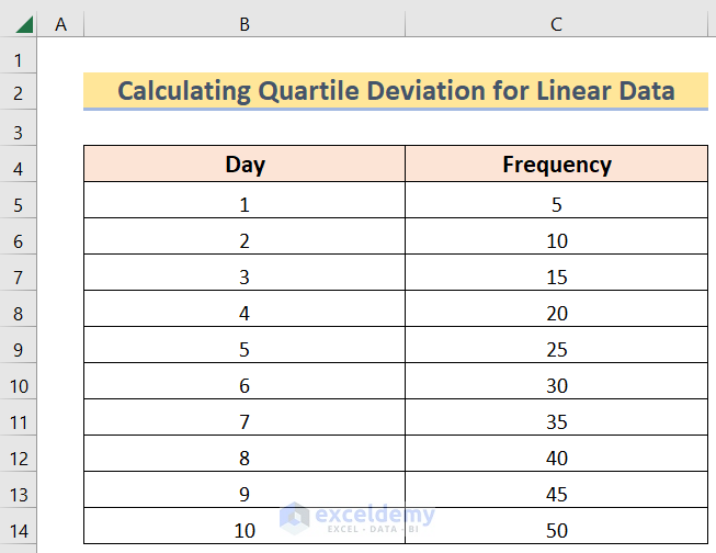
In this case, our goal is to calculate quartile deviation in Excel for linear data. That means we will have a sample dataset where we will have data for every certain heading. We can learn this method by following the below image.
Steps:
- First, arrange the dataset similarly to the below image. For instance, we have Day and Frequency in columns B and C.
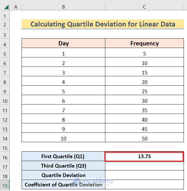
- Next, insert the following formula in the C16 cell.
=C6+0.75*(C7-C6)

- After that, you will get the First Quartile by using the above formula.
- Subsequently, insert the following formula in the C17 cell.
=C12+0.25*(C13-C12)
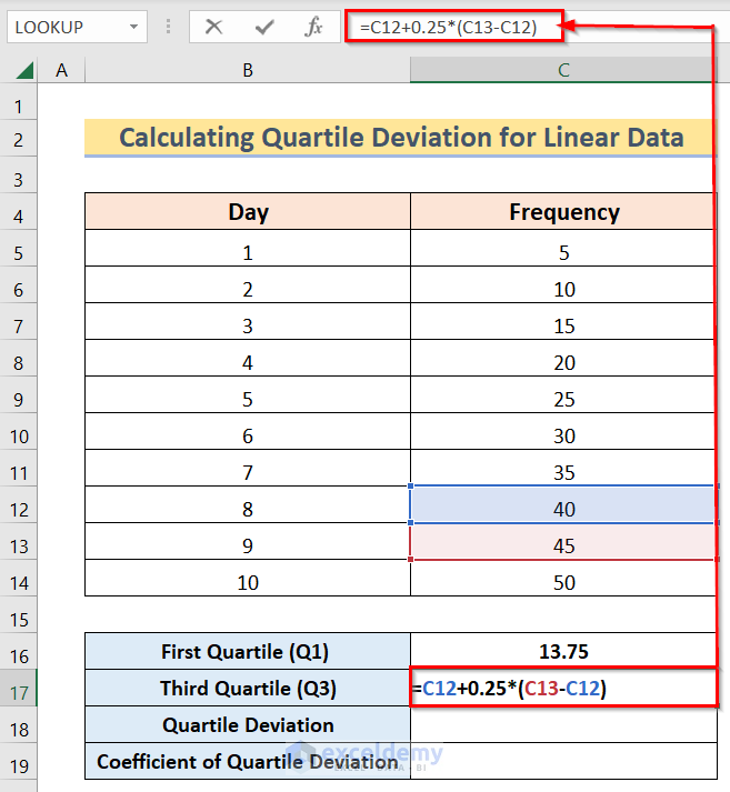
- Therefore, you will get the Third Quartile by using the above formula.

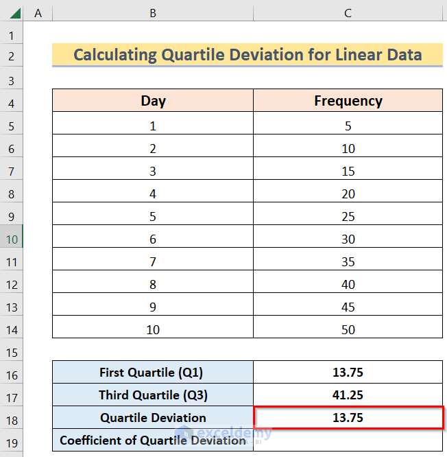
- Moreover, insert the following formula in the C18 cell.
=(C17-C16)/2

- Next, you will get the Quartile Deviation by using the above formula.
- In addition, insert the following formula in the C19 cell.
=(C17-C16)/(C17+C16)
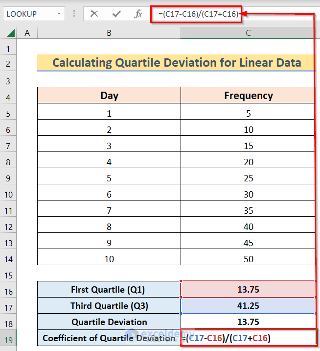
- Finally, you will get the Coefficient of Quartile Deviation by using the above formula.
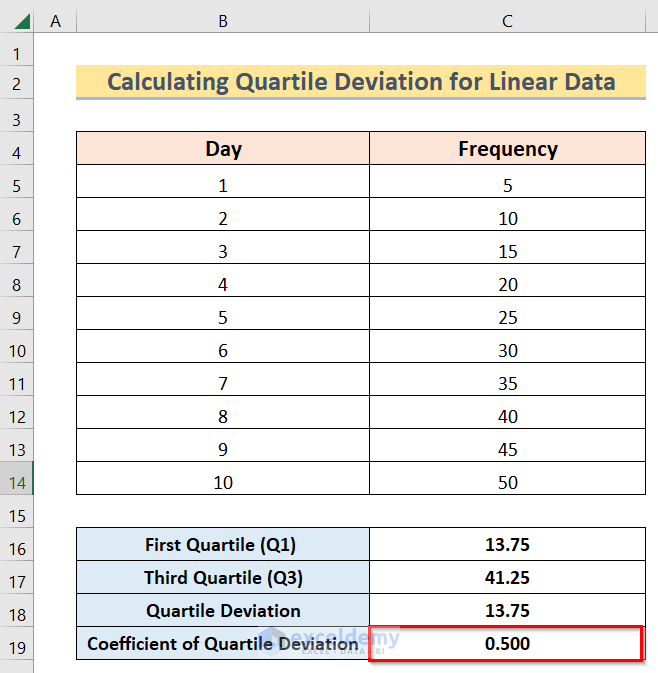
Hence, you have calculated the quartile deviation in Excel for linear data.
2. Determining Quartile Deviation for Grouped Data
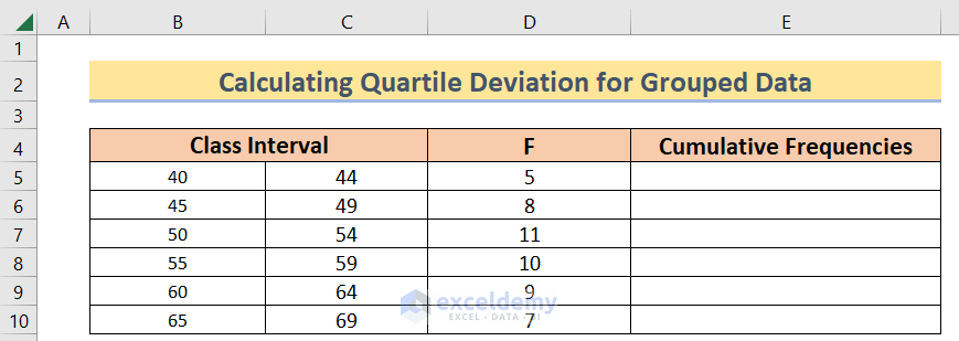
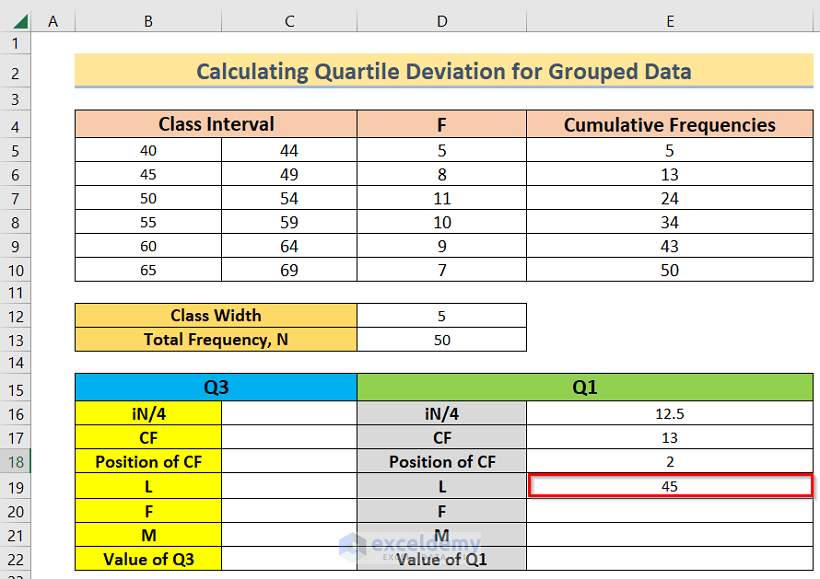
Now, we want to calculate the quartile deviation in Excel for grouped data. That means we will have a sample dataset where we will have ranged data that will have class intervals. We can learn this method by following the below image.
Steps:
- First, arrange the dataset like the image below. In this case, we have Class Interval in Column B, Frequency (F) in column D, and Cumulative Frequencies in column E.
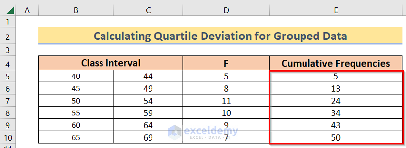
- Secondly, insert the following formula in the E5 cell.
=D5
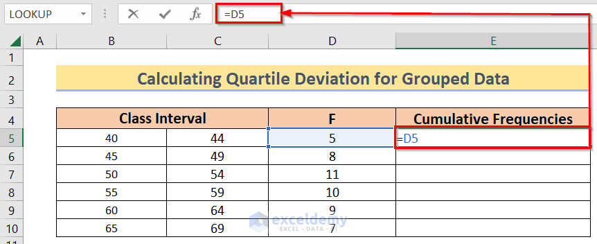
- Thirdly, you will get the first cumulative frequency which is the same as the first value of the frequency.

- Afterward, insert the following formula in the E6 cell.
=E5+D6
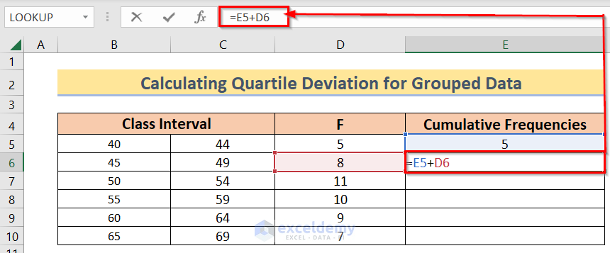
- Next to that, you will get the second cumulative frequency by adding the new frequency with the previous frequency.

- In addition, you will get the result for this cell and then use the Fill Handle to apply the formula to all cells.
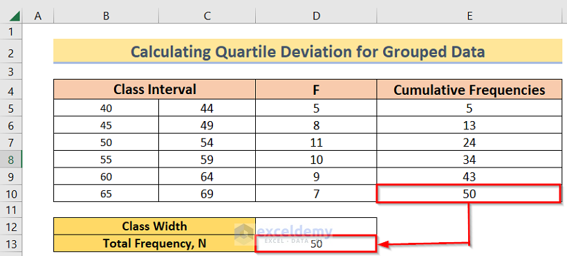
- Moreover, the Total Frequency will be the total value of Cumulative Frequency.
- Thereafter, insert the following formula in the D12 cell to calculate the Class Width.
=B6-B5
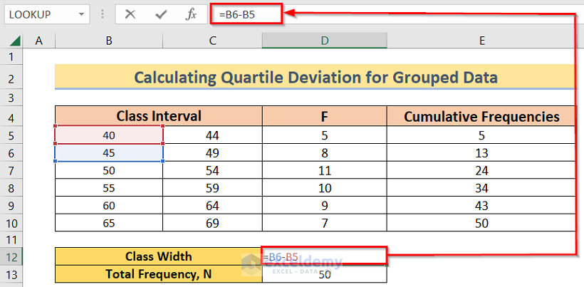
- Hence, you will get the result by subtracting the values.

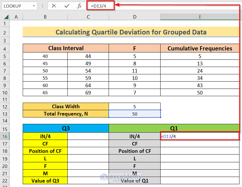
- Furthermore, to calculate the quartiles, you have to create two columns named Q1 and Q3. Each quartile consists of iN/4, CF, Position of CF, L, F, M, and Value of Q1 or Q3.

L presents the lower value of the interval that consists of the quartile cumulative frequency,
C represents the width of the class,
F represents the frequency of the interval,
N is the total frequency and
M is the cumulative frequency leading up to the interval.
- Along with this, insert the following formula in the E16 cell.
=D13/4
- Continuously, you will get the result by using division.

- Again, insert the following formula in the E17 cell.
=MIN(FILTER(E5:E10,E5:E10>=E16))
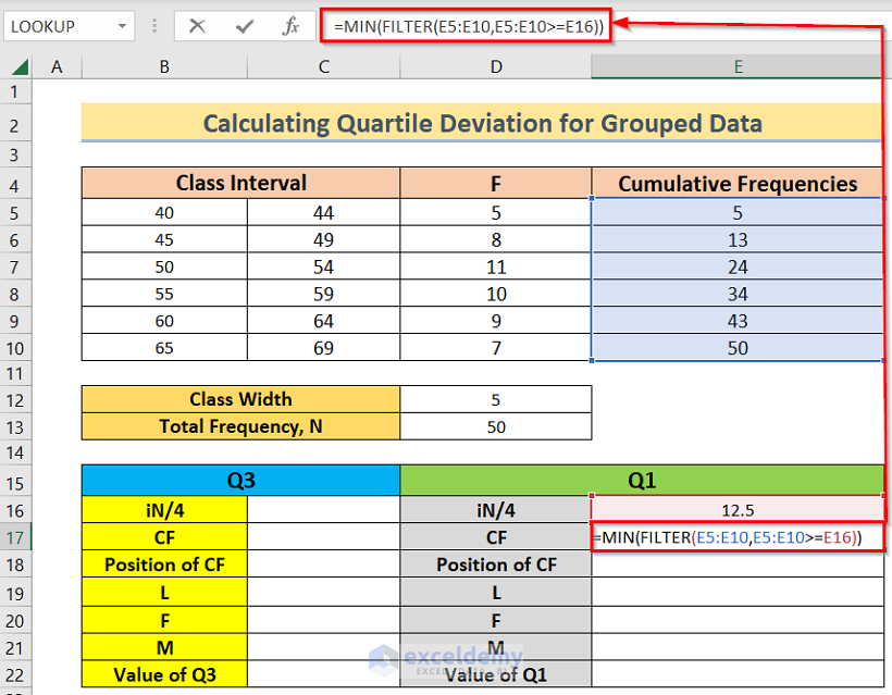
Note that, as we found (iN/4) value is 12.5 so we have filtered the E5 to E10 cells according to that condition by using the FILTER function and found the minimum value from it by using the MIN function.
- So, you will get the result by using a combination of MIN and FILTER So, you got result 13 in this case.

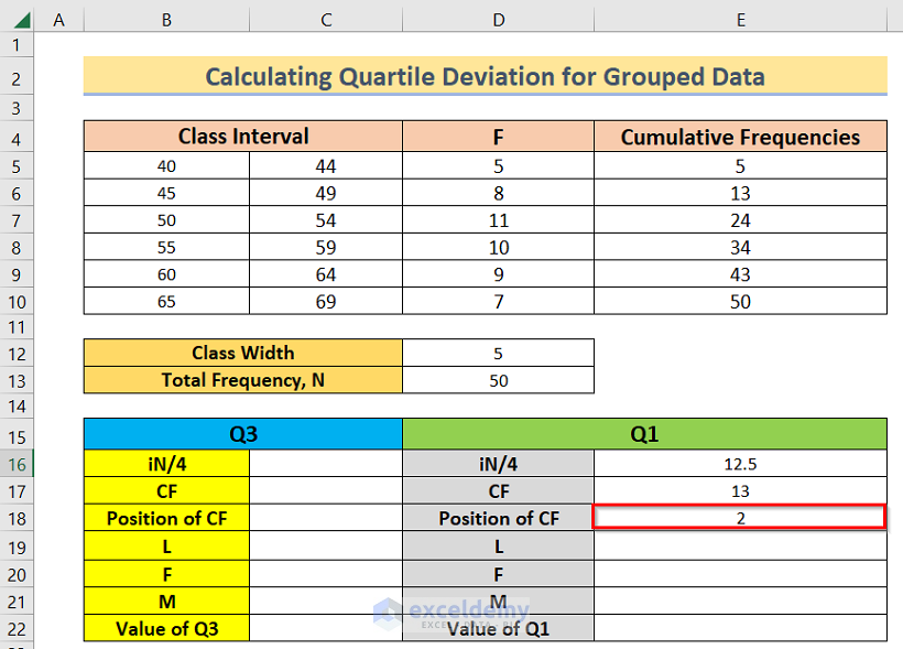
- Then, insert the following formula in the C18 cell.
=MATCH(E17,E5:E10,0)

Note, that we have the MATCH function to find the position of CF. We have applied the function on range E5 to E10 and it will look up with the help of the E17 cell.
- Next, you will get the result by using the MATCH function.
- After that, insert the following formula in the E19 cell.
=INDIRECT(ADDRESS(ROW(E4)+E18,2))
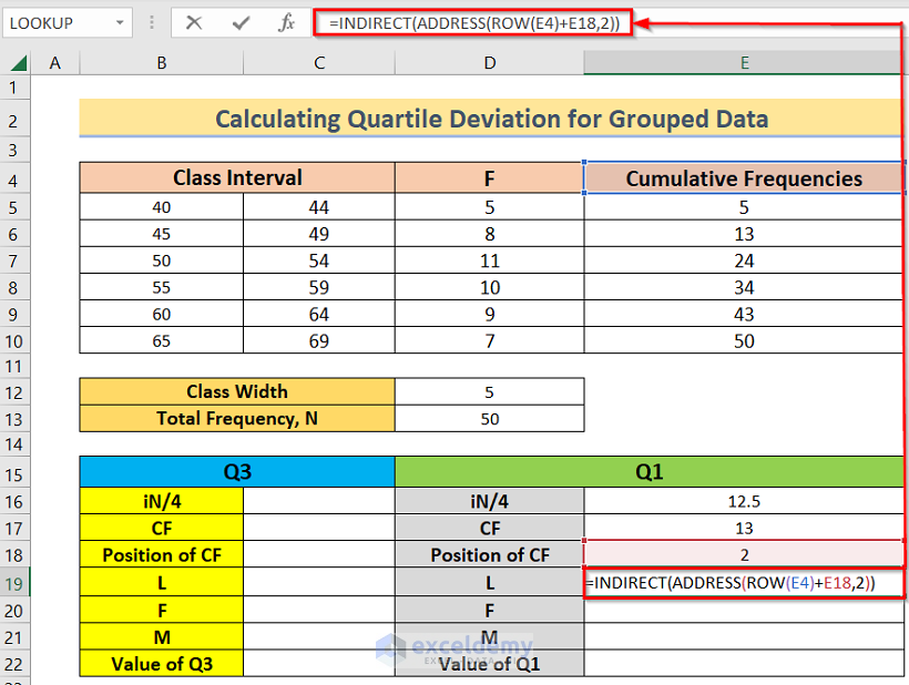
Note, first we have selected the rows by using the ROW function. After that, we used the ADDRESS function to select the row and column reference accordingly. And INDIRECT function shows the reference cells overall.
- Moreover, you will get the result by combining INDIRECT, ADDRESS, and ROW functions.
- Furthermore, insert the following formula in the E20 cell.
=INDIRECT(ADDRESS(ROW(E4)+E18,4))
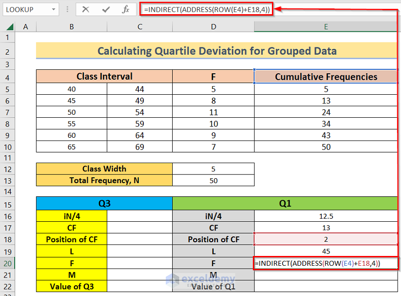
- Afterward, you will get the result by the combination of INDIRECT, ADDRESS, and ROW functions.

- Thereafter, insert the following formula in the E21 cell.
=INDIRECT(ADDRESS(ROW(E4)+E18-1,5))
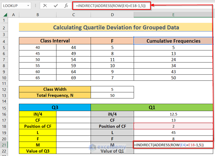
- Consequently, you will get the result by combining INDIRECT, ADDRESS, and ROW functions.

- Hence, insert the following formula in the E22 cell.
=E19+(D12/E20)*(E10/4-E21)
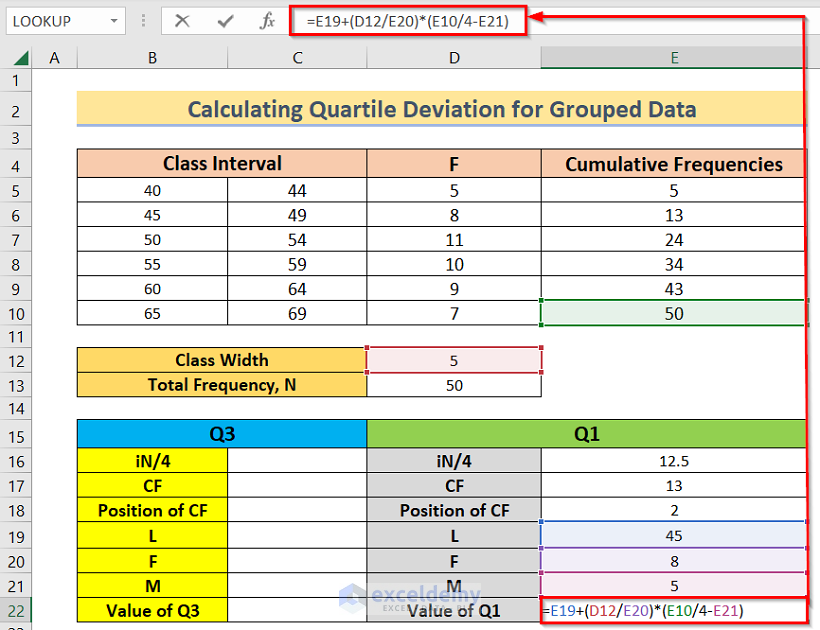
- As a result, you will get the Value of Q1 in the E22 cell.

- Subsequently, In this case, you need to multiply the new formula by 3 to find the third quartile. We will use the same formula as Q1 but this time we have to multiply by 3. The formula becomes, (iN/4)=3*D13/4=37. 5
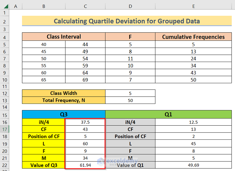
Then, if you repeat the same process, we will get the result for the Third Quartile of Q3 as well.
- Consequently, insert the following formula in the E24 cell.
=(C22-E22)/2
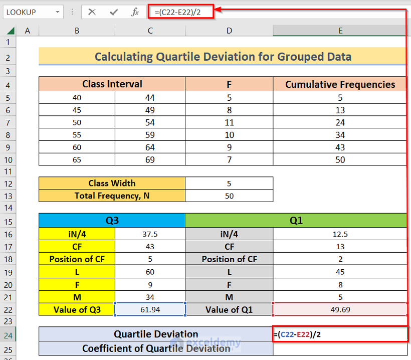
- Moreover, you will get the Quartile Deviation by using division.

- In addition, insert the following formula in the E25 cell.
=(C22-E22)/(C22+E22)

- Last, you will get the Coefficient of Quartile Deviation by using division.

Therefore, we have calculated the quartile deviation in Excel for grouped data.
Read More: How to Calculate Variance and Standard Deviation in Excel
3. Applying Excel QUARTILE.INC Function to Calculate Quartile Deviation
At this point, we want to calculate the quartile deviation in Excel by using QUARTILE.INC function. The QUARTILE.INC function is a built-in function in Excel that is categorized as a Statistical Function. Quartiles are values that split your data into quarters. It divides your data into four segments according to where the numbers fall on the number line. It is one of those essential functions. We can learn this method by following the below steps.
Steps:
- To begin with, arrange the dataset like the below image. In this case, we have Name in column B and Time in Column C. We want to find the Quartiles in Column E.

- In addition, insert the following formula in the F4 cell.
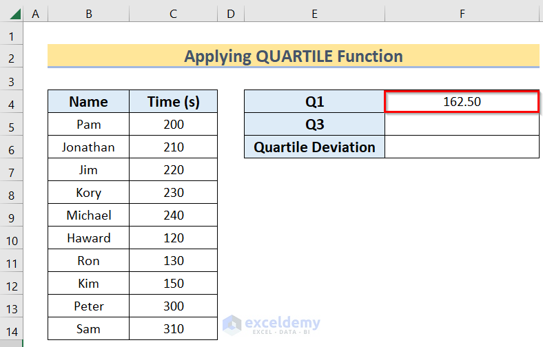
=QUARTILE.INC(C5:C14,1)
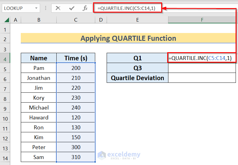
- Furthermore, you will get the result by using the First Quartile Q1.
- Moreover, insert the following formula in the F5 cell.
=QUARTILE.INC(C5:C14,3)

- Furthermore, you will get the result by using the Third Quartile Q3.

- Subsequently, insert the following formula in the F6 cell.
=(F5-F4)/2

- Finally, you will get the result by using the Quartile Deviation.

Read More: How to Calculate Absolute Deviation in Excel
4. Using AGGREGATE Function
Now, we want to calculate the quartile deviation in Excel by using the AGGREGATE function. In Excel, the AGGREGATE function is used on different functions to get specific results. We can learn this method by following the below steps.
Steps:
- First, arrange the dataset like the below image. We have Name and Marks in columns B and C.

- Secondly, insert the following formula in the C10 cell.
=AGGREGATE(17,4,C5:C9,1)

Note that The QUARTILE function accepts five values,
0 = Minimum value
1 = the First quartile, 25th percentile
2 = the Second quartile, 50th percentile
3 = the Third quartile, 75th percentile
4 = Maximum value
The function works with QUARTILE.INC (function number 17) and QUARTILE.EXC (function number 19) function to produce the quartile results.
- Thirdly, you will get the result by using the AGGREGATE function.

- Moreover, insert the following formula in the C11 cell.
=AGGREGATE(19,4,C5:C9,3)

- Consequently, you will get the result by using the EXC.

- Furthermore, insert the following formula in the C12 cell.
=(C11-C10)/2

- Lastly, you will get the result by using the Quartile Deviation.

Download Practice Workbook
You can download the practice workbook from here.
Conclusion
Henceforth, follow the above-described methods. These methods will help you to calculate quartile deviation in Excel. We will be glad to know if you can execute the task in any other way. Please feel free to add comments, suggestions, or questions in the section below if you have any confusion or face any problems. We will try our best to solve the problem or work with your suggestions.
Related Articles
<< Go Back to Deviation in Excel | Excel for Statistics | Learn Excel
Get FREE Advanced Excel Exercises with Solutions!
