Sometimes, we have to deal with a huge amount of data stored in several worksheets. In that case, we can mirror the cells in Excel instead of writing them on several occasions. There are 3 very simple ways to mirror cells in Excel with formula that we are going to discuss in this article. I hope this article will be helpful in lessening the workload and saving time.
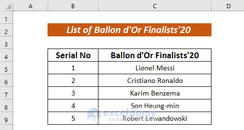
For more clarification, I have used a dataset on Ballon d’Or Finalists’20 in Serial No and Ballon d’Or Finalists’20 columns.
What Are Mirror Cells in Excel?
In general, the act of mimicking another person’s gesture, speaking pattern, or attitude is known as mirroring. But in Excel, Mirror cells mean linking cells across sheets in a defined pattern.
How to Mirror Cells with Formula in Excel: 3 Simple Ways
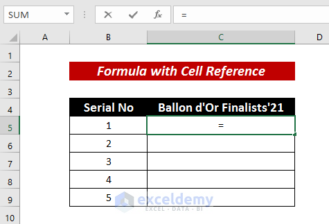
1. Formula with Cell Reference to Mirror Cells
The simplest way to mirror cells is to use the cell reference in the formula. In this way, we can create mirror across the sheets.
Steps:
- Select a cell in a new worksheet where you want to mirror cells. Here, I have created a worksheet named Cell Ref and selected cell C5 for mirroring.
- Then, input the Equal Sign (=) on that cell.
- Go to the sheet from where you want to mirror cells and select the cells. In my case, I went to the sheet named Ballon d’Or and selected cells from C5 to C9.
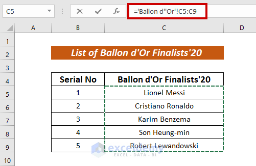
- Finally, press ENTER.
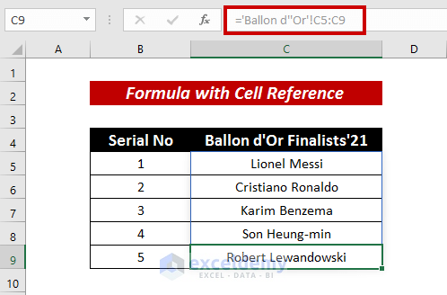
Thus, we can mirror cells across sheets.
2. Using INDIRECT and ROW Functions to Mirror Cells
There is another formula with a combination of the INDIRECT function and the ROW function to mirror cells. The whole procedure is mentioned below.
Steps:
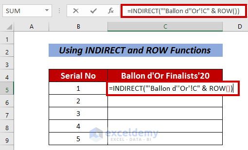
- Firstly, pick a cell in a new worksheet to mirror cells. Here, I have created a worksheet named INDIRECT and selected cell C5 for mirroring.
- Next, input the following formula.
=INDIRECT("'Ballon d''Or'!C" & ROW())Here, the ROW function identifies the row number. Then, it gets merged with strings inside the INDIRECT function and creates cell mirror.
- Press the ENTER button to have the output.
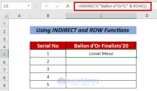
- Finally, use Fill Handle to AutoFill the rest cells.

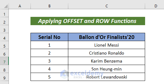
3. Applying OFFSET and ROW Functions to Mirror Cells
A combined formula with the OFFSET function and the ROW function can also be a terrific way to mirror cells. In this process, we can have the mirror cells in the opposite order.
Steps:
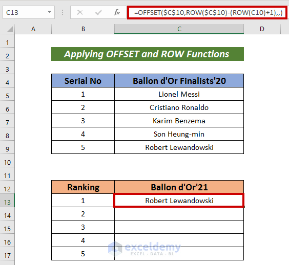
- I have created a dataset of the Ballon d’Or Finalists’20 in an order. But the Ballon d’Or’21 ranking was exactly in the opposite order.
- Create a new dataset to have the output in the opposite order.
- Next, input the following formula in that cell (i.e. C13).
=OFFSET($C$10,ROW($C$10)-(ROW(C10)+1),,)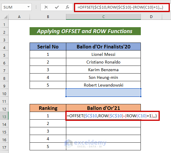
Formula Breakdown
ROW($C$10)-(ROW(C10)+1) —> Here, the ROW function returns the row number
Output: {-1}
OFFSET($C$10,ROW($C$10)-(ROW(C10)+1),,) —> The OFFSET function returns the cell value according to the number from the cell C10.
Output: Robert Lewandowski
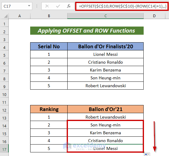
- Press ENTER to have the result.
- AutoFill the rest cells.
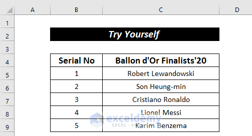
Practice Section
For more expertise, you can practice here.
Download Practice Workbook
Conclusion
That’s all for today. I have tried to explain 3 very simple ways to mirror cells in Excel with formula. It will be a matter of great pleasure for me if this article could help any Excel user even a little. For any further queries, comment below. You can visit our site for more articles about using Excel.
Related Articles
- How to Link Cells in Same Excel Worksheet
- How to Link Multiple Cells in Excel
- How to Link Multiple Cells from Another Worksheet in Excel
- How to Link Cells for Sorting in Excel
- How to Link Tables in Excel
- How to Stop Cell Mirroring in Excel
- How to Keep Formatting in Excel When Referencing Cells
- How to Automatically Link a Cell Color to Another in Excel
- How to Link Two Cells in Excel
<< Go Back To Excel Link Cells | Linking in Excel | Learn Excel
Get FREE Advanced Excel Exercises with Solutions!
