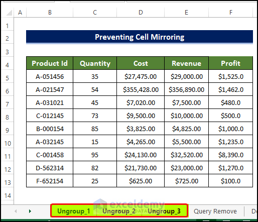
How to Stop Cell Mirroring in Excel (5 Easy Ways)

Method 1 – Ungrouping Worksheets

When multiple sheets in the workbook are grouped, entering data into any cell will input the same data into the same cell address across all of the grouped sheets. To resolve this, we need to ungroup the sheets.

Ungrouping Worksheets to Stop Cell Mirroring in Excel

Steps:

To ungroup a set group of sheets in Excel, right-click on any sheet in the grouped sheets.
Click on the Ungroup Sheets from the context menu.

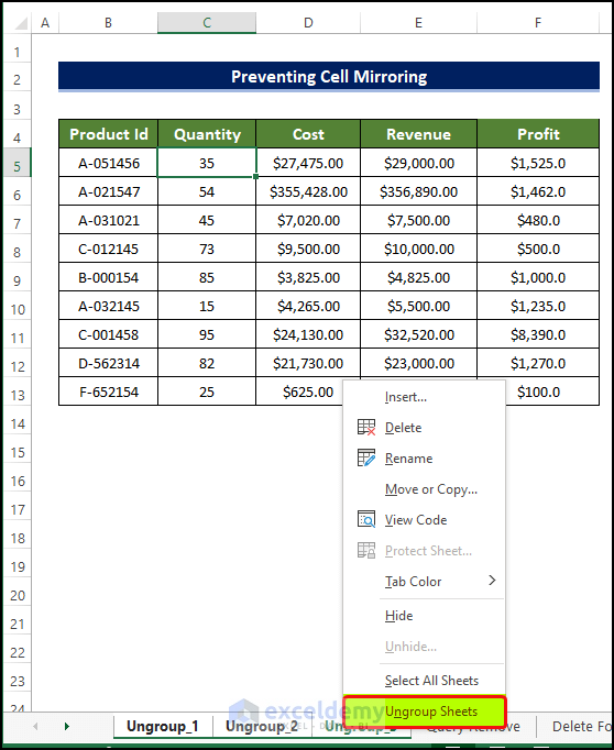
The mirroring of the cells in multiple sheets stops.
Entering anything in any of the Ungrouped cells results in change only in that cell.

Method 2 – Modify Formulas Across Worksheet

Steps:

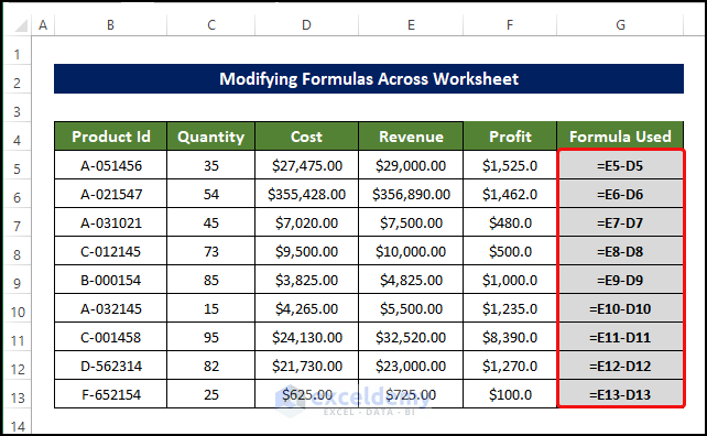
In the sample dataset below, the formula used in the range of cells G5:G13 is actually for the profit calculation. For Profit calculation, we have to subtract the Cost of good production from the Revenue earned.
We entered the formulas to calculate Profit in the range of cell G5:G13.
If we look at the formula distributions, then we can observe that there are some formulas that are displaced. And they need to be modified.

In the cells G6, G10 and G13, some formulas that are not supposed to be there.
As those range of cell values is supposed to calculate profit, we need to delete the Cost from the Revenue.

After modifying the highlighted formulas, cell monitoring will stop.

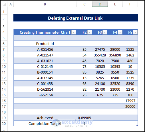
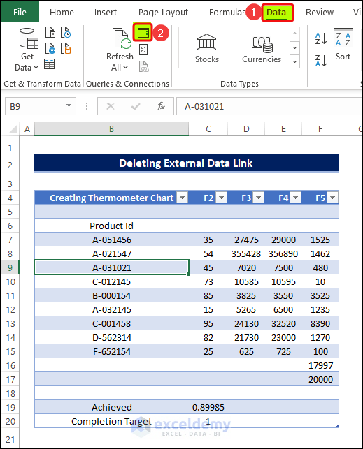
Method 3 – Delete External Data Link

If there is any external database, e.g., Excel is connected to another Excel workbook, any input in the source dataset will result in the data input in the destination dataset. To resolve this problem, the external data link needs to be deleted.

Steps:

Head to the Data tab, and click on Queries and Connections.

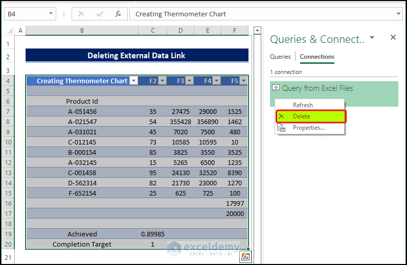
A new side panel named Queries and Connections opens.
Go to Connections segment >> right-click on Query from Excel Files and from the context menu click Delete.

There will be a warning sign, as shown below.

Click OK.

Method 4 – Prevent Cell Mirroring in Excel Table

In Excel tables, changing the formula in any cell affects the whole range of cells. To prevent this, we need to deactivate Autocorrect settings.

Steps:

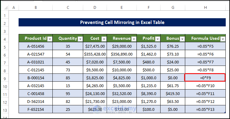
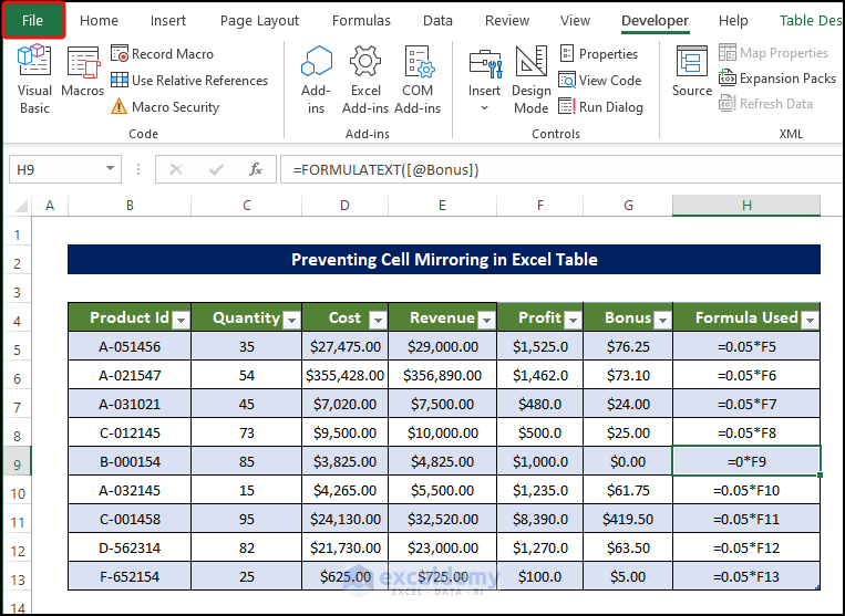
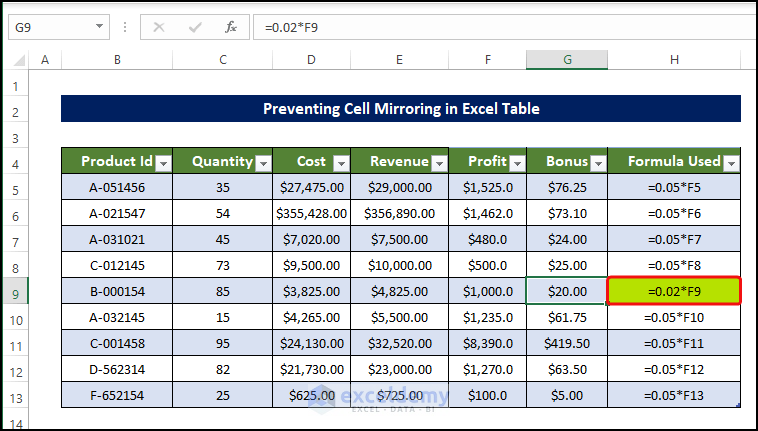
For example, we can observe that the formula used in the range of cells G5:G13, in the range of cells H5:H13.
They use the formula that estimates the Bonus which is 5% of the Profit.
But we have a new condition, the Bonus for Product B-000154 will be zero. Meaning the seller wouldn’t receive any profit for this product.
For this, we need to multiply 0.0 with F9 in cell G9 as shown in the image.

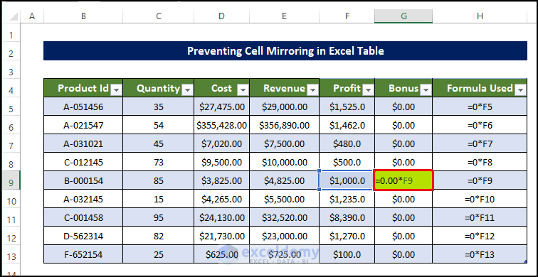
Press Enter after inputting the formula and we can see that all the other cells in the range of cells also multiply the Profit values with 0.
The result is that the whole range of cell G5:G13 is now showing 0.

Press Ctrl+Z, doing this will undo the previous step.
Which will bring back the original cell values, except for the cell we selected previously.

Cell G9 will show 0.0 as the formula suggested.
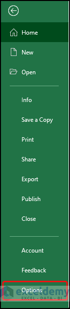
To resolve this issue, click on the File tab on the corner of the sheet.

From the Start menu, click on Options.

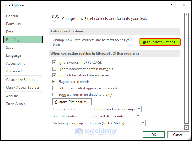
In the Excel Options dialog box, click on Proofing.
Click on the Autocorrect options.

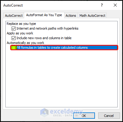
Autocorrect options dialog box opens.
Untick the Fill formulas in tables to create calculated columns.
Click OK.

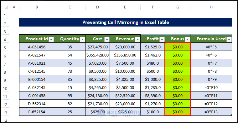
Enter 0.02 instead of 0.0 in the cell G9 formula.
You will notice that there is no change in the other cells in the range of cell G5:G13.

Method 5 – Apply User-Defined Function

Steps:

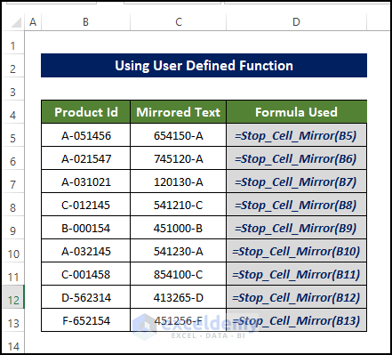
We have a sample dataset where the cell value is in reverse order.
The text value in the range of cell B5:B13 is now in the reverse order in the range of cell C5:C13.
You need to roll the text back to the original.
For this, we need a custom VBA function.

Go to the Developer tab and click on Visual Basic. If you don’t have that, you need to enable the Developer tab. Or You can also press ‘Alt+F11’ to open the Visual Basic Editor.

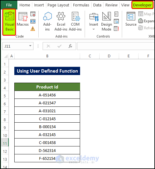
A new dialog box opens, click on Insert > Module.
Enter the following code:

Public Function Stop_Cell_Mirror(x As Range)
Stop_Cell_Mirror = StrReverse(x.Text)
End Function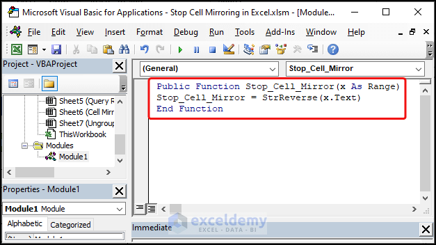

Close the Module
The custom function is set.
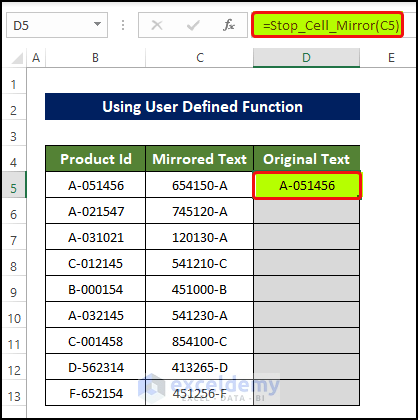
Select cell D5 and enter the following formula:

=Stop_Cell_Mirror(C5)

Entering this formula will reverse the order of the text in cell C5.

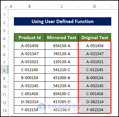
Drag the Fill Handle to cell D13.
Doing this will fill the range of cell D5:D13 with the reversed order or mirrored text of the range of cells C5:C13.