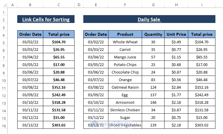
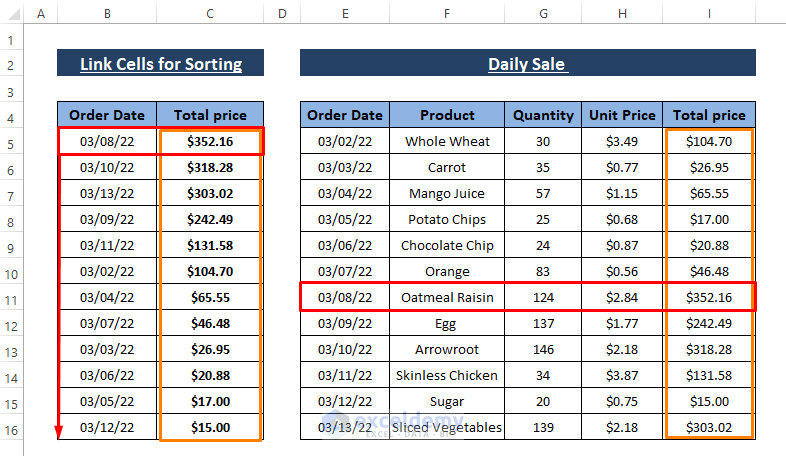
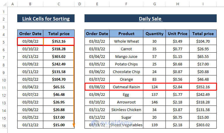
How to Link Cells for Sorting in Excel (5 Methods)

Sometimes we have to link cells in Excel for sorting or various purposes. Typical linking of a cell requires inserting an Equal sign (=) before a cell reference. However, linking cells with just equal signs results in discrepancies when sorting. Absolute Reference, functions like INDEX MATCH, VLOOKUP, XLOOKUP, and FILTER link the cells depending on criteria and solve sorting issues while linking cells.

Let’s say we have a Daily Sale dataset to which we want to link cells in the Link Cells for Sorting dataset.

In this article, we demonstrate multiple ways to link cells in Excel for sorting.

Issues with Linking Cells When Sorting

We normally link cells in Excel using an Equal Sign (=) and certain cell references as depicted in the below picture.

However, after linking cells if we execute sorting (Largest to Smallest) by the Home tab > Editing > Sort & Filter > Custom Sort, we see only the dates get sorted. Links cells don’t change their order though they are supposed to. This issue is shown in the following picture.

To resolve this issue, in the latter section we describe multiple ways.

How to Link Cells in Excel for Sorting: 5 Easy Ways

We link cells in a way that they can change their order with respective criteria (i.e., Date). As a result, the sorting issue can’t be a problem when each linked cell gets sorted along with its respective criteria. In the following methods, we first generate a lookup formula that doesn’t depend on rigid cell references and sort the linked cells afterward.

Method 1: Link Cells for Sorting Using Absolute Reference

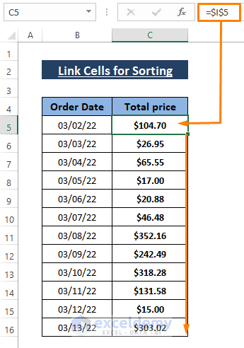
The easiest way to link any cell is by putting an Equal Sign before it with an Absolute References (i.e., =$I$11). The absolute reference keeps linked cells from breaking when Sorting.

Step 1: Insert Absolute References in cells of cells that you want to link to.

=$I$11

We want to link the C5 cell to the I5 cell. That’s why we put an absolute reference of cell I5.

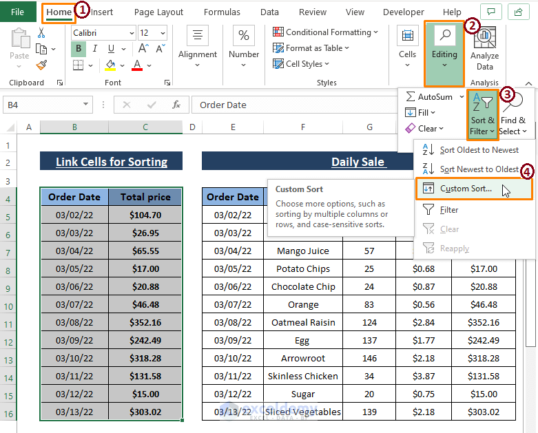
Manually input absolute references in all cells. It’s quite tiring; follow this method if you have only a handful of data unless don’t.

Step 2: Select the entire Link Cells for Sorting dataset, Go to the Home tab > Editing section > Select Sort & Filter > Choose Custom Sort.

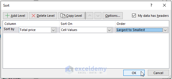
Step 3: The Sort command window pops up. In the window,

Choose Total Price as Sort by, Cell Values as Sort On, and Largest to Smallest as Order option.

Click on OK.

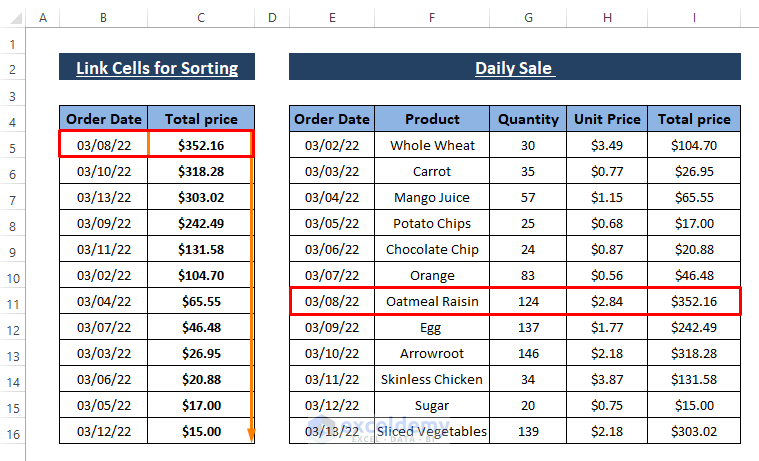
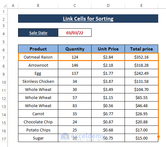
➤ In a moment, you see the highest Total Price cell values tops in the dataset along with the dates as shown in the below picture.

Inserting an Absolute Reference to solve sorting issues works and also links respective cells.

Method 2: Using INDEX – MATCH Functions to Link Cells for Sorting

Excel INDEX function finds a value of a given location within a given range. In our case, we use the MATCH function induced with the INDEX function. The MATCH function passes its result as a row number for entries that satisfy given criteria. The syntax of an INDEX function is

=INDEX(array, row_num, [col_num])

The MATCH function locates the position of a given value within a row, column, or table. As we said earlier, the MATCH portion passes the row number for the INDEX function. The syntax of the MATCH function is

MATCH (lookup_value, lookup_array, [match_type])

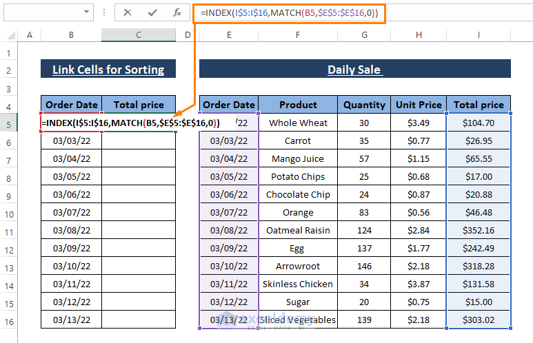
Step 1: Paste the below formula in any cell where you want to link the cell that satisfies the criteria.

=INDEX(I$5:I$16,MATCH(B5,$E$5:$E$16,0))

In the formula, I$5:I$16 refers to the array argument. The MATCH portion MATCH(B5,$E$5:$E$16,0) declares the row_num. And the MATCH portion assigns B5 as lookup_value, $E$5:$E$16 as lookup_array, and 0 declares the [match_type] as an exact match.

The used MATCH portion returns 1 as it finds 03/02/22 in row number 1 within the array.

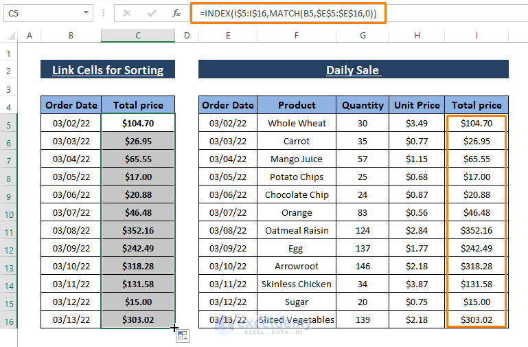
Step 2: Press ENTER and Drag the Fill Handle to apply the formula to other cells as picturized in the latter image.

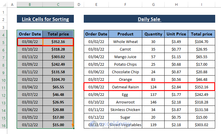
Step 3: Now, Repeat Steps 2 and 3 of Method 1 to execute Sorting. Afterward, you see Largest to Smallest sorting results in placing bigger values on tops. You can apply any of the Sorting options and static cell references won’t be an issue.

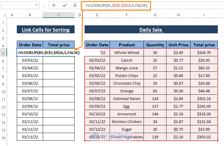
Method 3: Link Cells in Excel Using VLOOKUP Function

Similar to the INDEX MATCH operation, Excel VLOOKUP fetches entries depending on criteria. The syntax of the VLOOKUP function is

=VLOOKUP (lookup_value, table_array, column_index_num, [range_lookup])

Here,

lookup_value; The value Excel search within the 1^st column of the range or table.

table_array; The table from where you want to fetch the desired value.

column_index_num; The column number within the range or table you want to fetch a value.

[range_lookup]; By default, TRUE refers to an approximate match and FALSE refers to an exact match. [optional]

Step 1: Insert the following formula in any blank cell (i.e., C5).

=VLOOKUP(B5,$E$5:$I$16,5,FALSE)

In the formula,

B5 = lookup_value

$E$5:$I$16 = table_array

5 = column_index_num

FALSE = [range_lookup]

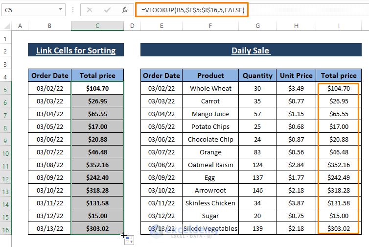
Step 2: Use the ENTER key to execute the formula and drag the Fill Handle to apply the formula in other cells.

Step 3: Again, Follow Steps 2 and 3 of Method 1 to execute sorting. In a moment, you see Largest to Smallest Sorting results in placing bigger values on tops as depicted in the below picture.

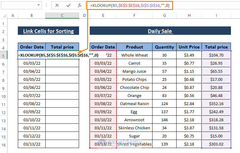
Method 4: Using XLOOKUP Function to Link Cells

Excel 365 offers a modern XLOOKUP function kind of similar to the VLOOKUP, HLOOKUP functions but enhanced in capabilities. The XLOOKUP function specifies arguments with respective ranges or arrays. The syntax of the XLOOKUP function is

=XLOOKUP (lookup, lookup_array, return_array, [not_found], [match_mode], [search_mode])

The arguments refer

lookup; The value you want to look for.

lookup_array; The range or array where to explore.

return_array; The range or array from where to return.

not_found; Return value in case no match is found. [optional]

match_mode; By default, exact match =0, an exact match or the next smallest =-1, an exact match or the next larger =1, a wildcard match = 2. [optional]

search_mode; By default, search from beginning = 1, search from last = -1, binary search in ascending order = 2, binary search in descending order = -2. [optional]

Step 1: Insert the following formula in any cell (i.e., C5).

=XLOOKUP(B5,$E$5:$E$16,$I$5:$I$16,"",0)

Comparing values to the arguments,

lookup = B5

lookup_array = $E$5:$E$16

return_array = $I$5:$I$16

[not_found] = “”

[match_mode] = 0

Step 2: Use the Fill Handle to apply the formula in other cells as shown in the below screenshot.

Step 3: Execute Steps 2 and 3 of Method 1 to apply Sorting and you see larger values placed on tops.

Method 5: Using FILTER Function to Fetch Required Columns for Sorting

Excel 365 also provides the FILTER function to fetch required columns for Sorting. The FILTER function can fetch arrays or ranges depending on its included argument. The syntax of the FILTER function is

FILTER (array, include, [if_empty])

array; The range or array you want to filter.

include; The criteria provided as Boolean array.

if_empty; The return value when no results are found. [optional]

To apply the FILTER function, we modify the dataset as shown in the below picture.

Step 1: Use the following formula to fetch particular columns.

=FILTER(H6:K16, G6:G16=C4)

The values in the formula refer

H6:K16 = array

G6:G16=C4 = include, works as criteria.

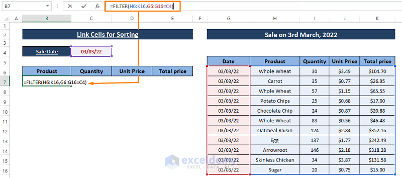
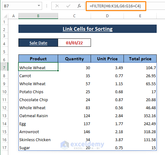
Step 2: Hit ENTER, Excel fetches all the required columns as shown in the below picture.

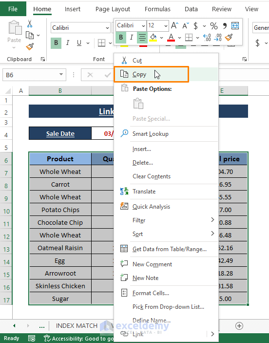
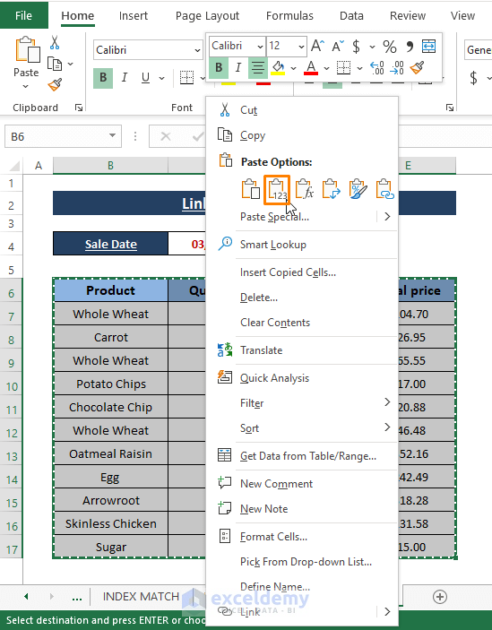
Step 3: Highlight the entire range, Right-Click on it. The Context Menu appears. In the Context Menu, Select Copy.

Step 4: Highlight the same range as you did in the previous step. Right-click on it. The Context Menu appears. From the Context Menu, Choose Paste Options Value.

Step 5: After pasting formulas as values use Steps 2 and 3 of Method 1 to apply Custom Sort by Total Price. Instantly, you can see the larger values get placed on tops.

You can choose other options offered in the Custom Sort window to execute Custom Sort. FILTER resultant values can’t be sorted as a result you must paste them as values in the range.

Download Excel Workbook

Link Cells for Sorting.xlsx

Conclusion

In this article, we demonstrate Absolute Reference, INDEX MATCH, VLOOKUP, XLOOKUP, and FILTER function to link cells in Excel for sorting. Absolute Reference and functions except FILTER link cells with ease and don’t break while sorting. However, the Copy and Paste operation needed to apply the FILTER function for sorting. Hope these above-mentioned methods excel in their objectives. Comment, if you have further inquiries or have anything to do.