Method 1 – Link Tables Using Pivot Tables in Excel
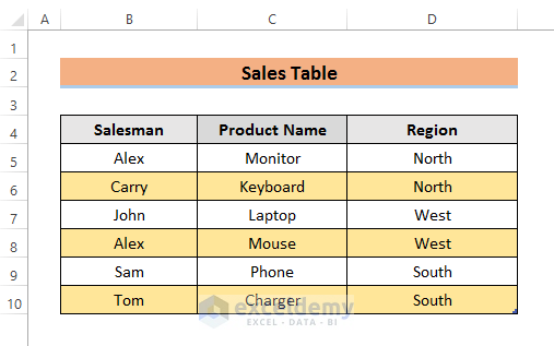
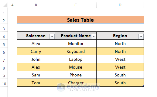
In our dataset, we will use two different tables from two different sheets. Sheet1 contains the Sales Table. This table has 3 columns. These are Salesman, Product Name, and Region.
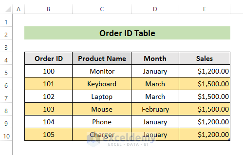
Sheet2 contains the Order ID Table. This table has 4 columns: Order ID, Product Name, Month, and Sales.
Steps:
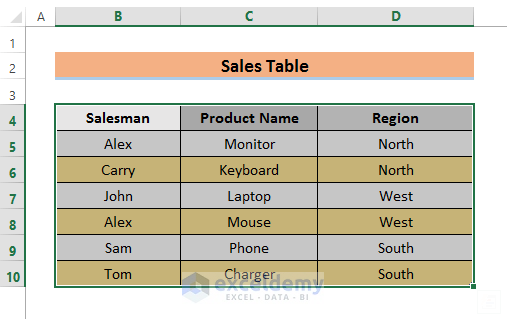
- We need to convert our dataset into a table. Select the range of cells in your dataset. We have selected the cells from B4 to D10.
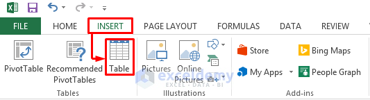
- Go to the INSERT tab and select Table.
- A Create Table window will appear. Make sure ‘My table has headers’ is selected.
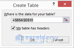
- Clicking OK will convert your dataset into a table just like below.
- Make an Order ID Table.

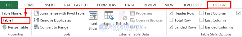
- Go to the DESIGN tab and change the name of the tables. We have changed Table1 to Sales and Table2 to Order.
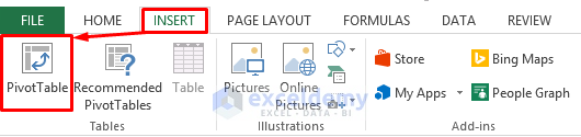
- Go to the INSERT tab and select Pivot Table.
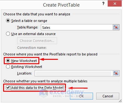
- A Create PivotTable window will pop up. Select ‘New Worksheet’ and ‘Add this data to the Data Model’. Do this for both tables.
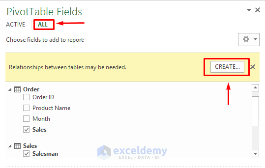
- A PivotTable Fields window will open. Select the columns you want to link from this window.
- Select Create.
- The Create Relationship window will open. Select the tables and columns you want to use for your relationship.
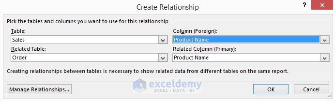
- Hit OK and a linked table will appear.

Read More: How to Link Multiple Cells from Another Worksheet in Excel
Method 2 – Apply Power Pivot to Link Tables
Steps:
- Activate the Power Pivot feature. Go to the FILE tab and select Options.
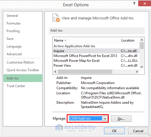
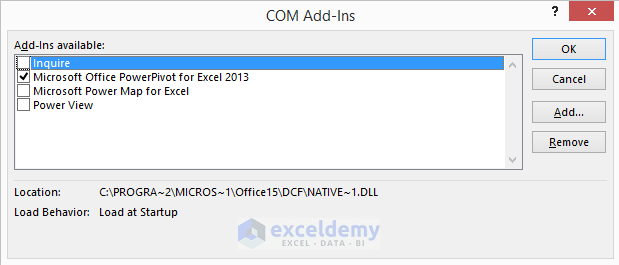
- The Excel Options window will appear. Go to the Add-Ins and select COM Add-ins.
- Select Go.
- A COM Add–Ins will open. Select ‘Microsoft Office PowerPivot for Excel 2013’ and click OK.
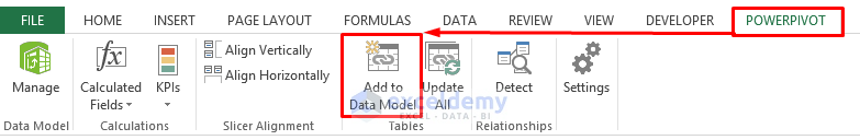
- Select the range of the data from your table.

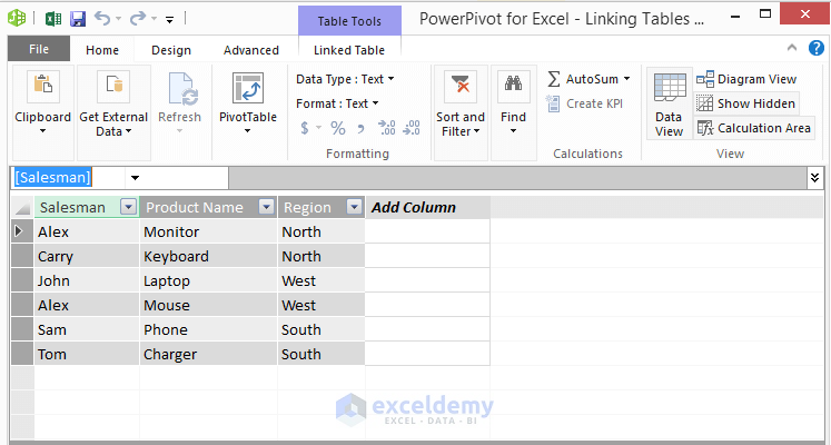
- Go to the POWERPIVOT ribbon and select Add to Data Model.
- A PowerPivot for Excel window will appear. Repeat the steps above for the Order Table.
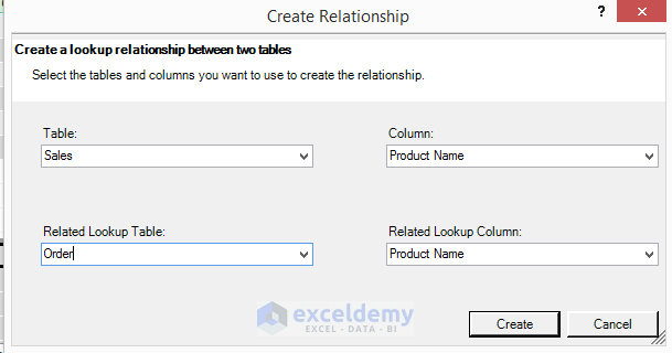
- Go to Design and select Create Relationship.
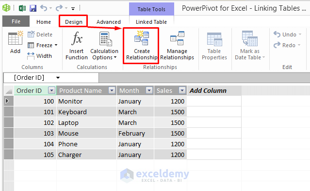
- Select the Table and Related Lookup Table for the linked table. You will have to use the same column in both tables for creating a relationship.
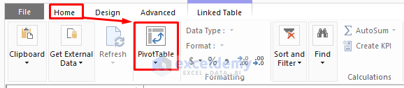
- Go to Home and select PivotTable.
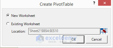
- A Create PivotTable window will occur. Select where you want to create the pivot table. We selected New Worksheet for this purpose. You can also select Existing Worksheet.
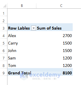
- Click OK and you will see the new table.
Read More: How to Link Cells in Same Excel Worksheet
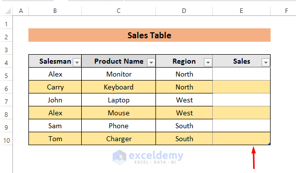
Method 3 – Link Multiple Tables Manually
We will use the previous tables for this method. The Sales column of the Order ID table will be added to the Sales table.
Steps:
- Add a Sales column beside the Region. This new column will be automatically added to the existing table.
- Insert this formula in E5.
=Sheet2!E5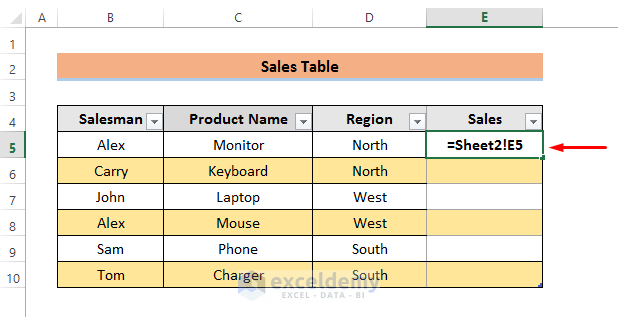
This formula will link the E5 cell from the Order ID table to our Sales table.
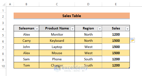
- Hit Enter and the whole column will be linked in the table.
Things To Remember
To link tables using the pivot table method, we need to have a common column in all tables. Otherwise, we can not create relationships. The PowerPivot feature is available from Excel 2013 version and later.
Download the Practice Book
Further Readings
- How to Link Multiple Cells in Excel
- Keep Formatting in Excel When Referencing Cells
- How to Link Cells for Sorting in Excel
- How to Stop Cell Mirroring in Excel
- How to Automatically Link a Cell Color to Another in Excel
- How to Link Two Cells in Excel
<< Go Back To Excel Link Cells | Linking in Excel | Learn Excel
Get FREE Advanced Excel Exercises with Solutions!
