Combining Excel SUMIF and VLOOKUP functions is one of the most popular formulas to gather values from multiple sheets and sum values based on a criterion. In this article, we are going to learn about how to do that with multiple examples and explanations. So, be prepared to go through the entire article.
Introduction to Excel SUMIF Function
The SUMIF function sums up the values based on a particular condition.
- Syntax:
=SUMIF(range, criteria, [sum_range])
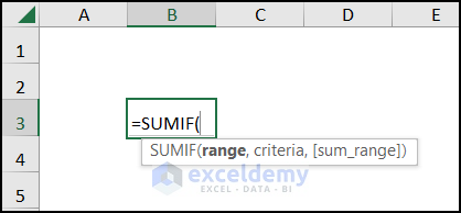
- Arguments:
range: The range of values to sum
criteria: Condition to use in the selected range
[sum_range]: Where we want to see the result.
Introduction to Excel VLOOKUP Function
The VLOOKUP function looks for a value in a vertically organized table and returns the matched value.
- Syntax:
=VLOOKUP (lookup_value, table_array, column_index_num, [range_lookup])
- Arguments:
lookup_value: It is the value that we want to look up.
table_array: From where we want to look.
column_index_num: The number of columns in the range containing the return value.
[range_lookup]: For exact match = FALSE, approximate / partial match = TRUE.
SUMIF and VLOOKUP Functions Across Multiple Sheets in Excel: 2 Easy Ways
1. Using SUMIF and VLOOKUP Functions Across Multiple Sheets
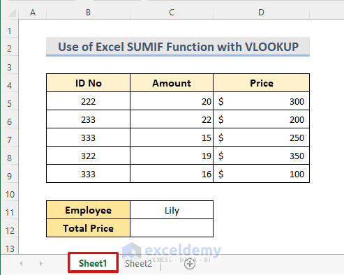
The SUMIF function works like the SUM function but it sums up only those values that match the given condition. So, we will use the VLOOKUP function inside the SUMIF function to input the criteria. Assuming we have two worksheets (Sheet1 and Sheet2). In Sheet1, we have all the employee’s ID No and their sales amount with the price in range B4:D9.
In Sheet2, we have all the employees’ names with their ID No.
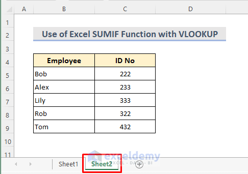
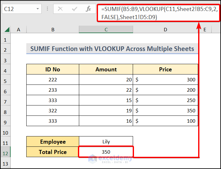
Here we are going to search for the employee Lily (Cell C11) of Sheet1. Presently, from Sheet2, we are going to look for her ID No and show the total sum of sales prices in cell C12 (Sheet1).
Steps:
- Select cell C12 in Sheet1 and type the formula.
=SUMIF(B5:B9,VLOOKUP(C11,Sheet2!B5:C9,2,FALSE),Sheet1!D5:D9)
- After that, hit ENTER to see the result.

Formula Breakdown
- VLOOKUP(C11,Sheet2!B5:C9,2,FALSE)
After that, this will look up the ID No for the value of Cell 11 of Sheet1 from Sheet2 cell range B5:C9. Then returns the exact match.
- SUMIF(B5:B9,VLOOKUP(C11,Sheet2!B5:C9,2,FALSE),Sheet1!D5:D9)
So, this will sum up all the prices, based on the exact match of ID No from the previous step.
Notes:
- If you’re not a Microsoft Office 365 user, then to get the final result, you have to press CTRL + SHIFT + ENTER as VLOOKUP works as an array formula.
- The column index number cannot be less than 1.
- SUMIF function only works on numerical data.
Read More: SUMIF for Multiple Criteria Across Different Sheet in Excel
2. Combining SUMIF, VLOOKUP & INDIRECT Functions Across Multiple Sheets
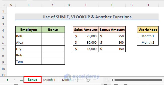
In this section, we are going to use SUMPRODUCT & INDIRECT functions with VLOOKUP & SUMIF functions for multiple worksheets. Here, we have three worksheets. At first, in the first worksheet Bonus, we can see the employee names. Then, we have to find out the amount of bonus for each employee. There is also a bonus criteria table (E4:F7) showing the bonus amount based on the sales amount. We need to extract values from Month 1 and Month 2 worksheets.
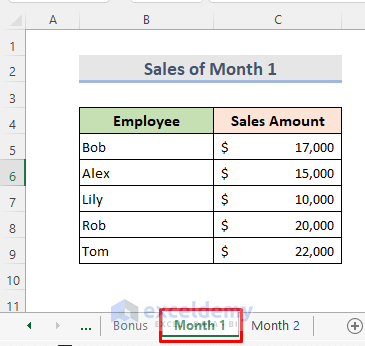
As a result, the sales of Month 1 are on the below worksheet.
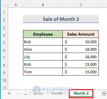
Therefore, the sales of Month 2 are on the below worksheet.
Steps:
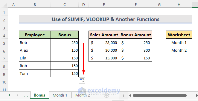
- Select cell C5 of the Bonus worksheet.
- Next, type the following formula:
=VLOOKUP(SUMPRODUCT(SUMIF(INDIRECT("'"&$H$5:$H$6&"'!"&"B5:B9"),Bonus!B5,INDIRECT("'"&$H$5:$H$6&"'!"&"C5:C9"))),$E$5:$F$7,2,TRUE)
- Hit ENTER and use Fill Handle to see the rest of the result.
Formula Breakdown
- The INDIRECT function converts the text string into a valid cell reference. Here it will refer to the sheets from range H5:H6.
- To include the range of sum and criteria, the SUMIF function will use reference worksheets that we indicated. It will return the value sales amount of each employee from the worksheets Month 1 & Month 2.
- The SUMPRODUCT function will sum up the amounts we found from the above procedure.
- In the Bonus worksheet, the VLOOKUP function looks up from range E5:E7. At last, it will return the matched bonus amount of an employee.
Notes:
- The column index number won’t be less than 1.
- Input the index number as a numerical value.
- SUMIF function only works on numerical data.
- We should press Ctrl+Shift+Enter as VLOOKUP works as an array formula.
Read More: Sum Based on Column and Row Criteria in Excel
Download Practice Workbook
Download the following workbook and do the exercises.
Conclusion
That’s all about today’s session. So, these are some easy methods to combine SUMIF and VLOOKUP functions across multiple sheets in Excel. Please let us know in the comments section if you have any questions or suggestions. For a better understanding, please download the practice sheet. Visit our website to find out about diverse kinds of Excel methods. Thanks for your patience in reading this article.
Related Readings
- SUMIF with Multiple Criteria in Different Columns in Excel
- How to Apply SUMIF with Multiple Ranges in Excel
- How to Sum Multiple Columns Based on Multiple Criteria in Excel
<< Go Back to SUMIF Multiple Criteria | Excel SUMIF Function | Excel Functions | Learn Excel
Get FREE Advanced Excel Exercises with Solutions!

i have multiple sheets in which the sum column range is in different columns. in one sheet it is k, in another it is l in another it is aa column etc. How will you change the sum column reference in the formula
If you are interested in answering this please do so. Dpont tell me that i have to pay 50 Dollers or 20 dollers etc
Dear S. NARASIMHAN,
Thanks for your valuable comment. No, you do not need to pay any amount of dollars to have your question answered.
To clarify your query, I have considered a case where I have Product Name in B5:B9 but their sales value is in different columns in 3 different sheets. For sheet named January, the sales amount is in D5:D9 and for February & March sheets, the sales amounts are in E5:E9 & G5:G9. Followingly, I have applied the following formula to find the total sales value of iPhone.
=SUM(VLOOKUP(D12,$B$5:$D$9,{3},FALSE),VLOOKUP(B5,February!$B$5:$E$9,{4},FALSE),VLOOKUP(B5,March!$B$5:$G$9,{6},FALSE))Here, D12 refers to the product name which is to look for in the Product Name column, and return output from Sales to have the summation. As you can see in the formula, I have used {3}, {4}, and {6} to define the column having sales amount referring to the first column of the look-up range as 1.
I hope you have your desired output from the above discussion.
Your Regards,
Naimul Hasan Arif