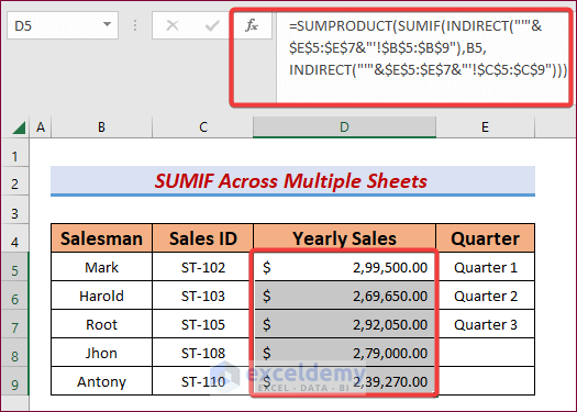
In our datasheet, we have Quarterly sales by different salesmen across different sheets. Now we want to calculate the yearly sales of different salesmen. For that, we have to sum up the different quarters’ sales of each salesman.
Method 1 – Using SUMIF Function for Each Sheet
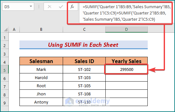
Suppose we want to calculate the yearly sales of each salesman in a sheet named Sales Summary:
- Type the following formula in cell D5:
=SUMIF('Quarter 1'!B5:B9,'Sales Summary'!B5,'Quarter 1'!C5:C9)+SUMIF('Quarter 2'!B5:B9,'Sales Summary'!B5,'Quarter 2'!C5:C9)+SUMIF('Quarter 3'!B5:B9,'Sales Summary'!B5,'Quarter 3'!C5:C9) Here,
‘Quarter 1′!B5:B9’ = Range in sheet Quarter 1 where the criteria will be matched.
‘Sales Summary’!B5′ = Criteria.
‘Quarter 1′!C5:C9’ = Range in sheet Quarter 1 from where value for summation will be taken.
In a similar manner, SUMIF is used for all of the sheets.
- After pressing Enter, you will get the summation of all three quarters’ sales of Mark in cell D5.
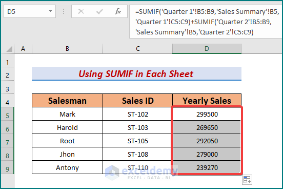
- Drag the sales D5 to the end of your dataset and you will get the yearly sales of all salesmen.
Read More: SUMIF for Multiple Criteria Across Different Sheet in Excel
Method 2 – Merging SUMPRODUCT SUMIF and INDIRECT Functions Across Multiple Sheets
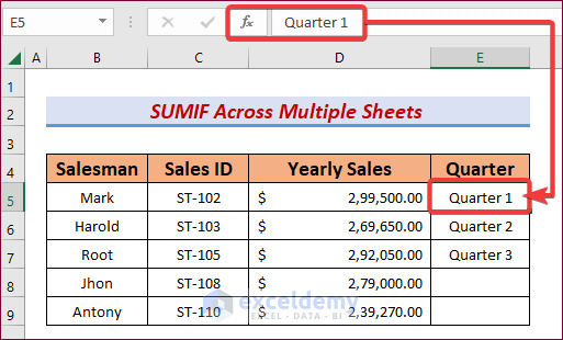
- Insert the name of the sheets (Quarter 1, Quarter 2, Quarter 3) in the sheet where we will make the calculation for yearly sales.
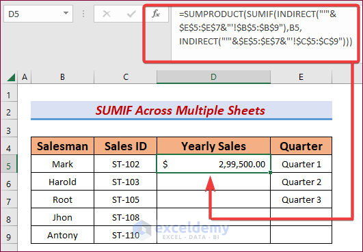
- Type the following formula in cell D5.
=SUMPRODUCT(SUMIF(INDIRECT("'"&$E$5:$E$7&"'!$B$5:$B$9"),B5,INDIRECT("'"&$E$5:$E$7&"'!$C$5:$C$9")))
- $E$5:$E$7 = refers to different sheets for the values of quarterly sales.
- B$5:$B$9 = lookup range for criteria.
- B5 = the criteria (Mark).
- $C$5:$C$9 = range for value if criteria match.
- Press Enter to get the summation of all three quarters’ sales of Mark in cell D5.
- Drag the sales D5 to the end of your dataset and you will get the yearly sales of all salesmen.
Method 3 – Utilizing VBA to Implement SUMIF Across Multiple Sheets
- Press Alt+ F11 to open the VBA window.
- Right-click on the sheet name and select Insert, then Module.

- A code window will appear. Copy and paste the following code into this window:
Function SUMIFOS(lookup_value As Range, ParamArray cellranges() As Variant)
Dim i As Integer, rng1 As Variant, temp As Single, a As Boolean
Dim rng2 As Variant, value As Variant, j As Single
If (UBound(cellranges) + 1) Mod 2 <> 0 Then
  Exit Function
End If
For i = LBound(cellranges) To UBound(cellranges) Step 2
    If cellranges(i).Rows.Count <> cellranges(i + 1).Rows.Count Then
    End If
    If cellranges(i).Columns.Count <> 1 Then
        Exit Function
End If
    rng1 = cellranges(i).value
    rng2 = cellranges(i + 1).value
    For j = LBound(rng1) To UBound(rng1)
        For Each value In lookup_value
            If UCase(rng1(j, 1)) = UCase(value) Then a = True
        Next value
        If a = True Then temp = temp + rng2(j, 1)
        a = False
    Next j
Next i
SUMIFOS = temp
End Function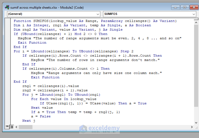
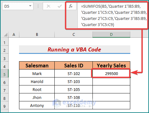
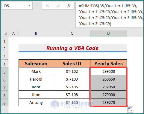
- Close the VBA window and type the following formula in cell D5:
=SUMIFOS(B5,'Quarter 1'!B5:B9,'Quarter 1'!C5:C9,'Quarter 2'!B5:B9,'Quarter 2'!C5:C9,'Quarter 3'!B5:B9,'Quarter 3'!C5:C9)Here, SUMIFOS is the custom function, B5 is the lookup value, Quarter 1′!C5:C9 is the range for value in the sheet named Quarter 1, and Quarter 1′!B5:B9 is the range for criteria in the sheet named Quarter 1. You can insert the value from as many sheets as you want in this formula.
- After pressing Enter, you will get the summation of all three quarters’ sales of Mark in cell D5.
- Drag the sales D5 to the end of your dataset and you will get the yearly sales of all salesmen.
Read More: How to Apply SUMIF with Multiple Ranges in Excel
Download Practice Workbook
Related Articles
- How to Sum Based on Column and Row Criteria in Excel
- SUMIF with Multiple Criteria in Different Columns in Excel
<< Go Back to SUMIF Multiple Criteria | Excel SUMIF Function | Excel Functions | Learn Excel
Get FREE Advanced Excel Exercises with Solutions!

Hi. These Sumif and Indirect functions were very helpful for my project. In fact, I started to use some.. However, I don’t know how to use the function to get the sum of two columns in multiple sheets using sumif and indirect. It will only sum one column.
For example, the datas to be summed were in column D and E. when using the sumif and indirect function with 1 column, the formula perfectly works well. Like E:E.. But when I try to include the D column like D:E, it will turn out zero.
Please help.
Hello KC,
Thanks for the feedback. It appears that the INDIRECT function is unable to return the sum of two columns from multiple worksheets, even though it works fine for a single column. Rather, we can use the XLOOKUP and SUM functions to get the results.
You can download the Excel file included in this reply.
SUMIF Across Multiple Sheets.xlsx
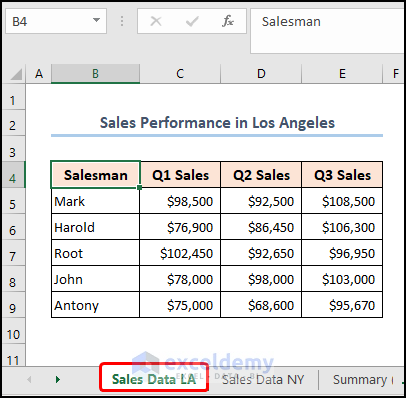
Consider the Sales Performance dataset for Los Angeles, likewise, we have the Sales Performance dataset for New York.
The screenshot below shows the aggregate sales for each salesman using the SUM and XLOOKUP functions.
=SUM(XLOOKUP(B5,'Sales Data LA'!$B$4:$B$9,'Sales Data LA'!$C$4:$E$9),
XLOOKUP(B5,'Sales Data NY'!$B$4:$B$9,'Sales Data NY'!$C$4:$E$9))
Regards,
ExcelDemy