This is an overview:
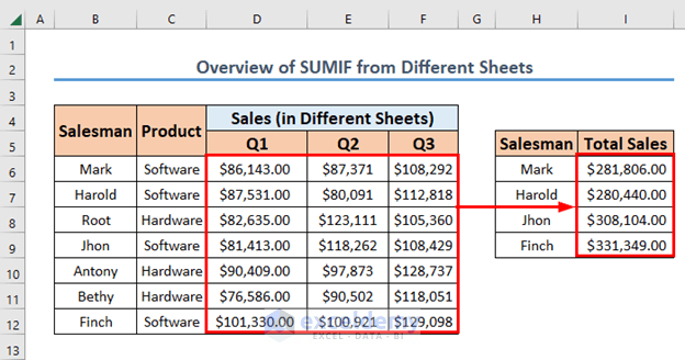
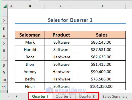
The sample dataset showcases records of quarterly sales in three different sheets: Quarter 1, Quarter 2, and Quarter 3. Two different types of products are sold: Software and Hardware.
To calculate the yearly sales of software in a new sheet (Sales Summary):
Method 1 – Using the SUMIF Function to Sum values in Different Sheets with Multiple Criteria
Steps:
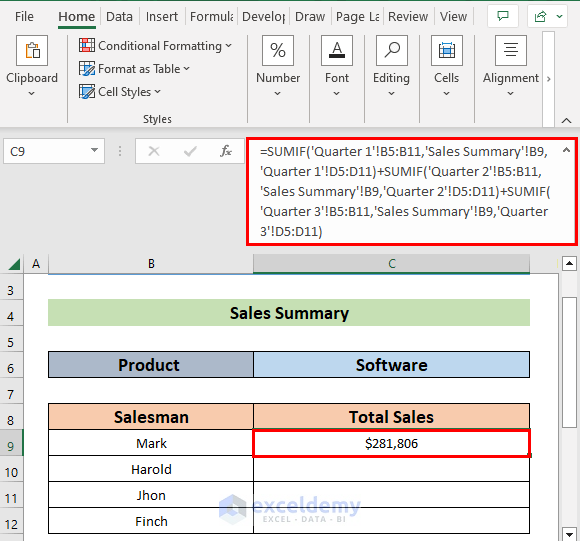
- Go to C9 and enter the following formula.
=SUMIF('Quarter 1'!B5:B11,'Sales Summary'!B9,'Quarter 1'!D5:D11)+SUMIF('Quarter 2'!B5:B11,'Sales Summary'!B9,'Quarter 2'!D5:D11)+SUMIF('Quarter 3'!B5:B11,'Sales Summary'!B9,'Quarter 3'!D5:D11)- Press ENTER to see the output.
Formula Breakdown
- Quarter 1′!B5:B11 is the range for criteria in Quarter 1.
- Sales Summary’!B9 is the criteria in Sales Summary.
- Quarter 1′!D5:D11 is the range for the value in the Quarter 1 sheet.
- the SUMIF function is applied to the two other sheets.
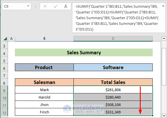
- Drag C9 to get the summation of Software sales in the three quarters for the other salesmen.
Read More: SUMIF Across Multiple Sheets in Excel
Method 2 – Usineg the SUMIFS Function to Sum in Different Sheets with Multiple Criteria
To sum different quarter Software sales in a new sheet (Sales Summary-2).
Steps:
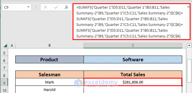
- Go to C9 and enter the following formula.
=SUMIFS('Quarter 1'!D5:D11,'Quarter 1'!B5:B11,'Sales Summary-2'!B9,'Quarter 1'!C5:C11,'Sales Summary-2'!$C$6)+ SUMIFS('Quarter 2'!D5:D11,'Quarter 2'!B5:B11,'Sales Summary-2'!B9,'Quarter 2'!C5:C11,'Sales Summary-2'!$C$6)+SUMIFS('Quarter 3'!D5:D11,'Quarter 3'!B5:B11,'Sales Summary-2'!B9,'Quarter 3'!C5:C11,'Sales Summary-2'!$C$6)- Press ENTER to see the output.
Formula Breakdown
- Quarter 1′!D5:D11 is the sum range in the Quarter 1 sheet,
- Quarter 1′!B5:B11 is the range for criteria 1 in the Quarter 1 sheet,
- Sales Summary-2′!B9 is the first criteria in the Sales Summary-2 sheet,
- Quarter 1′!C5:C11 is the range for criteria 2 in the Quarter 1 sheet,
- ‘Sales Summary-2’!$C$6 is the second criterion in Sales Summary-2,
- The SUMIFS function is applied to the two other sheets.
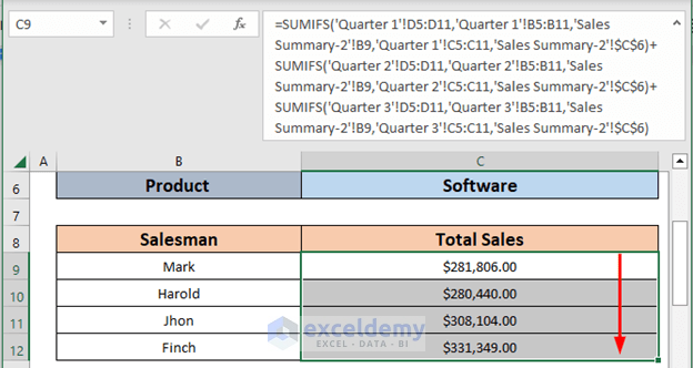
- Drag down the Fill Handle to AutoFill the formula.
Read More: SUMIF Multiple Ranges
Method 3 – Using the SUMPRODUCT, the SUMIFS and the INDIRECT Functions
Steps:
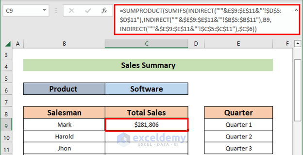
- Insert a new sheet (Sales Summary-3).
- Go to C9 and enter the following formula.
=SUMPRODUCT(SUMIFS(INDIRECT("'"&E$9:$E$11&"'!$D$5:$D$11"),INDIRECT("'"&$E$9:$E$11&"'!$B$5:$B$11"),B9,INDIRECT("'"&$E$9:$E$11&"'!$C$5:$C$11"),$C$6))- Press ENTER to see the output.
Formula Breakdown
- “‘”&E$9:$E$11&”‘!$D$5:$D$11” → references Sales.
- Output: {“‘Quarter 1’!$D$5:$D$11″;”‘Quarter 2’!$D$5:$D$11″;”‘Quarter 3’!$D$5:$D$11”}
- “‘”&$E$9:$E$11&”‘!$B$5:$B$11” → references Salesmen.
- Output: {“‘Quarter 1’!$B$5:$B$11″;”‘Quarter 2’!$B$5:$B$11″;”‘Quarter 3’!$B$5:$B$11”}
- “‘”&$E$9:$E$11&”‘!$C$5:$C$11” → references Product Category.
- Output: {“‘Quarter 1’!$C$5:$C$11″;”‘Quarter 2’!$C$5:$C$11″;”‘Quarter 3’!$C$5:$C$11”}
- INDIRECT(“‘”&$E$9:$E$11&”‘!$B$5:$B$11”) → is the criteria_range1.
- Output: {“Antony”;”Antony”;”Antony”}
- INDIRECT(“‘”&$E$9:$E$11&”‘!$C$5:$C$11”) → is the criteria_range2
- Output: {“Hardware”;”Hardware”;”Hardware”}
- SUMPRODUCT(SUMIFS(INDIRECT(“‘”&E$9:$E$11&”‘!$D$5:$D$11”),INDIRECT(“‘”&$E$9:$E$11&”‘!$B$5:$B$11”),B9,INDIRECT(“‘”&$E$9:$E$11&”‘!$C$5:$C$11”),$C$6)) → becomes,
- SUMPRODUCT({86143;87371;108292})
- Output: 281806
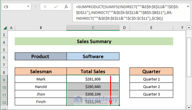
- Drag down the Fill Handle to see the result in the rest of the cells.
Download Practice Workbook
Further Readings
- SUMIF with Multiple Criteria in Different Columns in Excel
- How to Sum Based on Column and Row Criteria in Excel
<< Go Back to SUMIF Multiple Criteria | Excel SUMIF Function | Excel Functions | Learn Excel
Get FREE Advanced Excel Exercises with Solutions!
