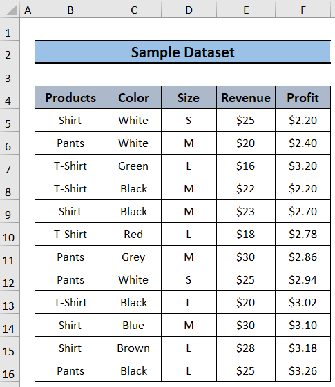
This is the sample dataset:
Method 1 – Using the SUMIF Function with a Single Criterion
Steps:
- Select I6 and enter the formula below.
=SUMIF($B$5:$B$16,H4,E5:E16)- Press Enter.
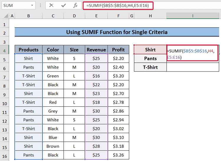
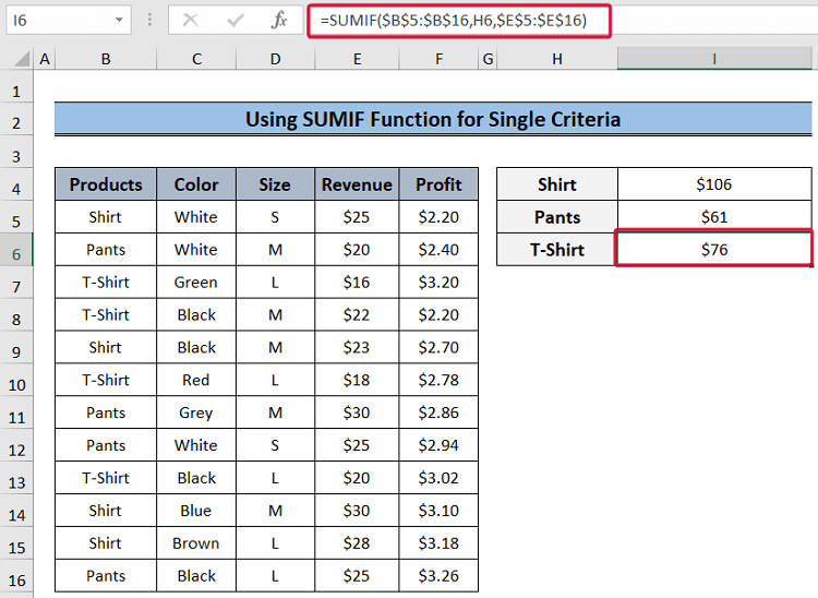
You will see the total revenue of the product T-Shirt.
- Repeat the procedure to find the values of Pants and Shirt.
Formula Breakdown:
- SUMIF($B$5:$B$16,H4,E5:E16): goes through B5:B16 to look for the value in H6 (T-shirt). It sums all values in E5:E16 and returns the sum.
Method 2 – Using the SUMIF function with Multiple Criteria
2.1. Applying the OR Logic
Steps:
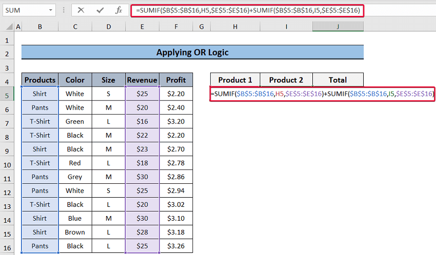
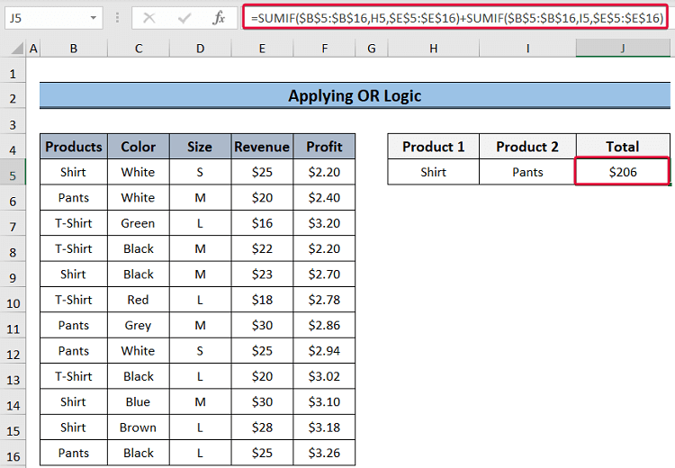
- Select J5 and enter the formula below.
=SUMIF($B$5:$B$16,H5,$E$5:$E$16)+SUMIF($B$5:$B$16,I5,$E$5:$E$16)- Press Enter.
This is the output.
Formula Breakdown:
- SUMIF($B$5:$B$16,H5,$E$5:$E$16): returns the sum of the revenues associated with the value in H5 (Shirt).
- SUMIF($B$5:$B$16,I5,$E$5:$E$16): returns the sum of values associated with Pants in E5:E16.
- SUMIF($B$5:$B$16,H5,$E$5:$E$16)+SUMIF($B$5:$B$16,I5,$E$5:$E$16): sums the values returned by the previous expressions.
2.2. Using an Array within the SUM Function
Steps:
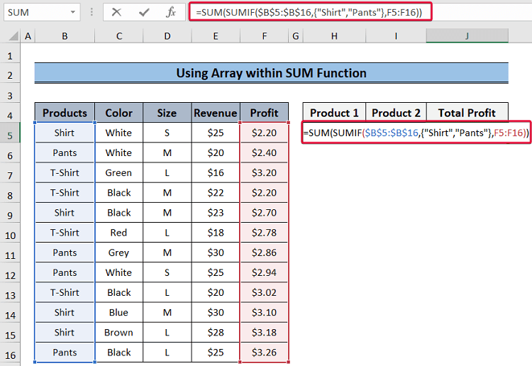
- Select J5 and enter the formula below.
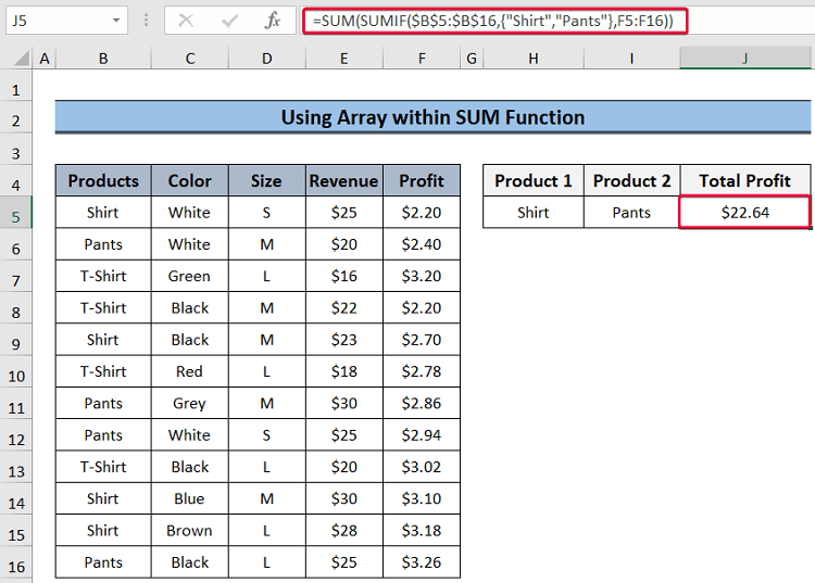
=SUM(SUMIF($B$5:$B$16,{"Shirt","Pants"},F5:F16))- Press Enter.
- This is the output.
Formula Breakdown:
- SUMIF($B$5:$B$16,{“Shirt”,”Pants”},F5:F16): goes through B5:B16 to look for Shirts and Pants. It sums the profit of these products in F5:F16 and returns it as the input for the SUM function.
- SUM(SUMIF($B$5:$B$16,{“Shirt”,”Pants”},F5:F16)): returns the sum of the profit.
2.3. Applying an Array Formula
Steps:
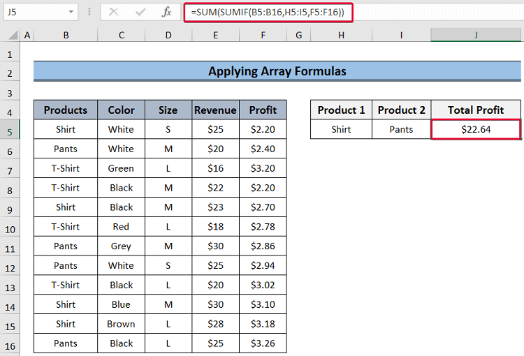
- Select J5 and enter the formula below.
=SUM(SUMIF(B5:B16,H5:I5,F5:F16))- Press Enter.
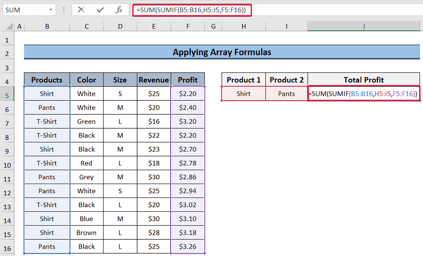
This is the output.
Formula Breakdown:
- SUMIF(B5:B16,H5:I5,F5:F16): The values in H5:I5 are the criteria. The function goes through B5:B16 to look for the criteria and sum the values individually. It returns the values as arguments for the SUM function.
- SUM(SUMIF(B5:B16,H5:I5,F5:F16)): sums the values returned by the SUMIF function.
2.4. Using an Array with the SUMPRODUCT Function
Steps:
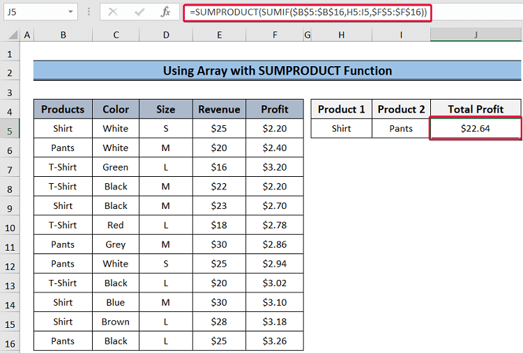
- Select J5 and enter the formula below.
=SUMPRODUCT(SUMIF($B$5:$B$16,H5:I5,$F$5:$F$16))- Press Enter.
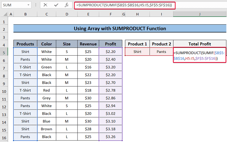
This is the output.
Read More: SUMIF for Multiple Criteria Across Different Sheet in Excel
Method 3 – Using the SUMIFS function with Multiple Criteria
Steps:
- Select J5 and enter the formula below.
=SUMIFS($E$5:$E$16,$B$5:$B$16,H5,$C$5:$C$16,I5)- Press Enter.
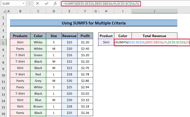
This is the output.
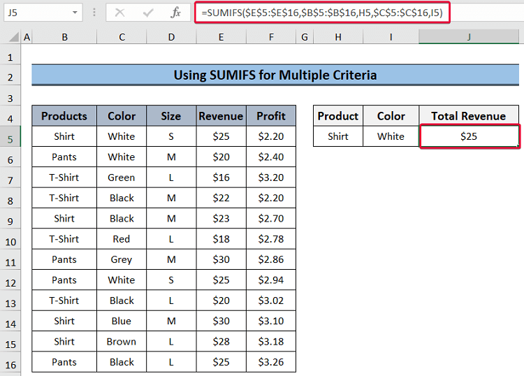
Formula Breakdown:
- SUMIFS($E$5:$E$16,$B$5:$B$16,H5,$C$5:$C$16,I5): The first argument, $E$5:$E$16, is the sum range of the function (revenue). The second argument, $B$5:$B$16, is the criteria range for the first criterion (Shirt in H5). The last two arguments are the second criteria range and the second criterion. The function looks for shirts in the first criteria range and white in the second. It returns the total revenue of white shirts.
Read More: How to Apply SUMIF with Multiple Ranges in Excel
Download Practice Workbook
Download the practice workbook.
Related Articles
<< Go Back to SUMIF Multiple Criteria | Excel SUMIF Function | Excel Functions | Learn Excel
Get FREE Advanced Excel Exercises with Solutions!

Method 2 has two problems. First, the example formula you ask us to type was pasted in wrong, with a nonsensical expression after the second `=` sign.
Second and more importantly, this method double-counts any value that matches both criteria. As such, it only works in cases where you know the two criteria will never overlap.
Hello Peter S,
Thank you for catching this. You were right that the formula shown in Method 2 contained an error. We’ve corrected the formula and removed the unintended expression that appeared after the second SUMIF function. We appreciate your careful review and feedback, which helped us improve the accuracy of the article.
Regards,
ExcelDemy