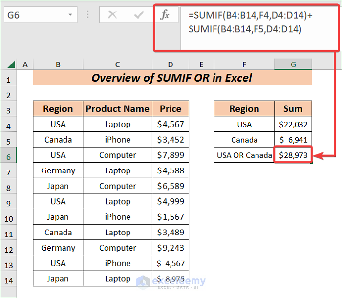
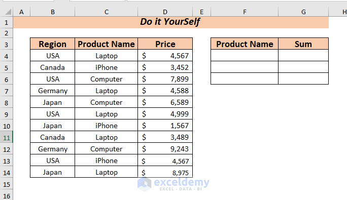
How to Use the SUMIF with OR Logic in Excel (10 Methods)

Below is a dataset of sales information. The dataset has three columns: Region, Product Name, and Price. Each column represents the sales amount of a particular product in a different region.

Method 1 – Using Multiple SUMIF with OR

Steps:

Select the cell where you want to place your result.
Enter the following formula:

=SUMIF(B4:B14,F4,D4:D14)+SUMIF(B4:B14,F5,D4:D14)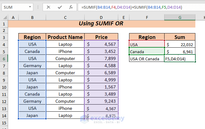

I wanted the sum from the USA or Canada, so I used these two regions as criteria. In the first SUMIF function, the USA is the criterion given in range B4:B14 to extract the sum from the sum_range D4:D14. Then, I wrote the SUMIF function again, using criteria Canada was given the range B4:B14 within the sum_range D4:D14.
To apply OR logic, add both separate SUMIF formulas.

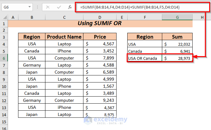
Press the ENTER key. You will see that the formula summed the values for the USA and Canada using OR logic.

Method 2 – Using Multiple SUMIF with OR on Different Columns

Steps:

Select the cell where you want to place your resultant value.
Enter the following formula:

=SUMIF(B4:B14,F4,D4:D14)+SUMIF(C4:C14,G4,D4:D14)

Here, I want to sum up the price for the laptop or product from the USA region. So, I’ve used the criteria USA from the Region column and Laptop from the Product Name column. In the first SUMIF function, the USA is the criterion given in range B4:B14 to extract the sum from the sum_range D4:D14. Then, I wrote the SUMIF function again, using the criteria Laptop and given the range B4:B14, where the sum_range was D4:D14.
To apply OR logic, add both separate SUMIF formulas.

Press the ENTER key. The formula will sum the values of two different columns using OR logic.

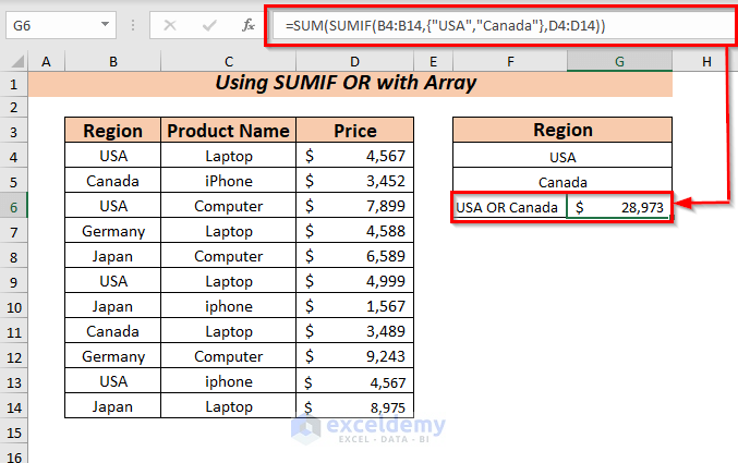
Method 3 – Using SUM within SUMIF OR with an Array

Steps:

Select the cell to place your resultant value.
Enter the following formula:

=SUM(SUMIF(B4:B14,{"USA","Canada"},D4:D14))

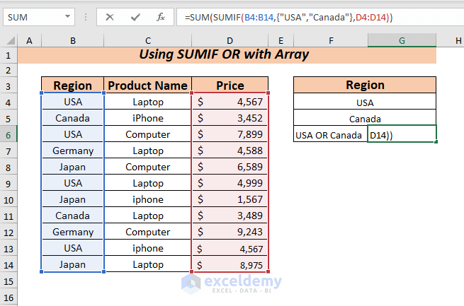Here, I used the USA and Canada as criteria. Now, the SUMIF function takes the USA and Canada as an array in the criteria given the range B4:B14 and where the sum_range is D4:D14. Then, it will sum the values if at least one of the conditions/criteria is met.

Press the ENTER key. The formula that summed the values when one criterion was fulfilled will appear.

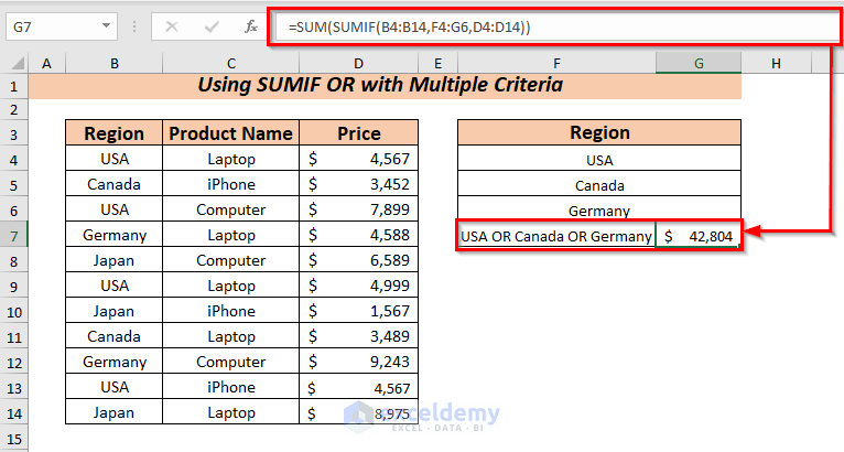
Method 4 – Using SUMIF OR with Multiple Criteria

Steps:

Select the cell to place your resultant value.
Enter the following formula:

=SUM(SUMIF(B4:B14,F4:G6,D4:D14))

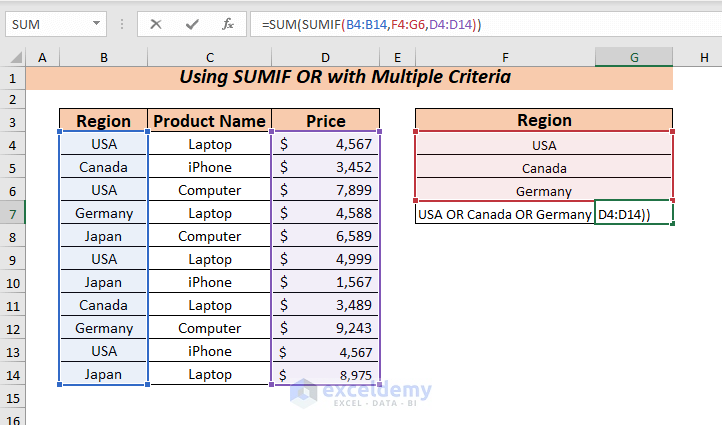Here, I used the USA, Canada, and Germany as criteria. Now, in the SUMIF function, I took the criteria range F4:G6 given the range B4:B14 to generate a sum from the sum_range D4:D14.

Then, the SUM function will sum the values if at least one of the conditions/criteria is met.

Press the ENTER key. You will see that the used formula summed the values for the criteria range.

Method 5 – Using SUMIF OR with SUMPRODUCT

Steps:

Select the cell to place your resultant value.
Enter the following formula:

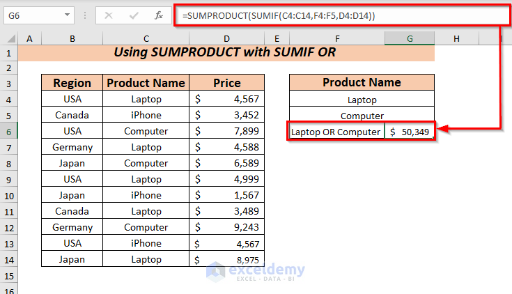
=SUMPRODUCT(SUMIF(C4:C14,F4:F5,D4:D14))

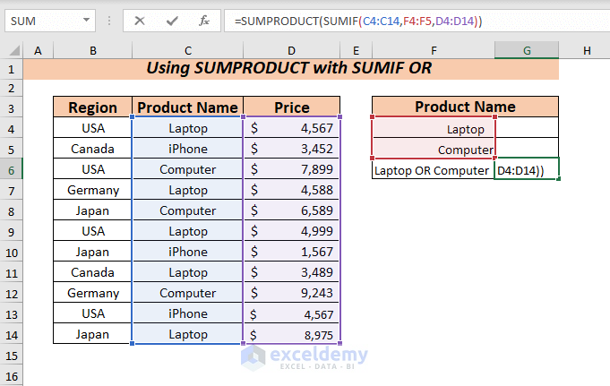Here, as I want to sum the Price for the product Laptop or Computer, I’ve used the Laptop and Computer from the Product Name column as criteria. Now, in the SUMIF function, I took the criteria range F4:F5 given the range C4:C14, where the sum_range was D4:D14. Then, the SUMPRODUCT function will sum the values if at least one of the conditions/criteria is met.

Press the ENTER key. You will see that the used formula summed the values for the criteria range.

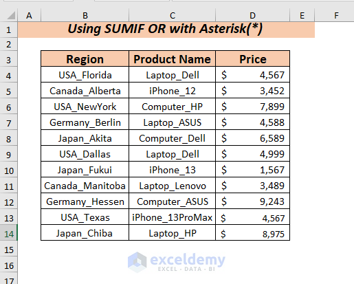
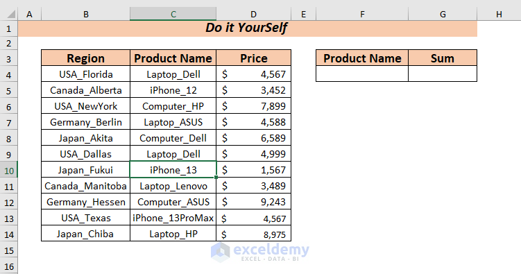
Method 6 – Using SUMIF OR with Asterisk (*)

Steps:

Select the cell to place your resultant value.
Enter the following formula:

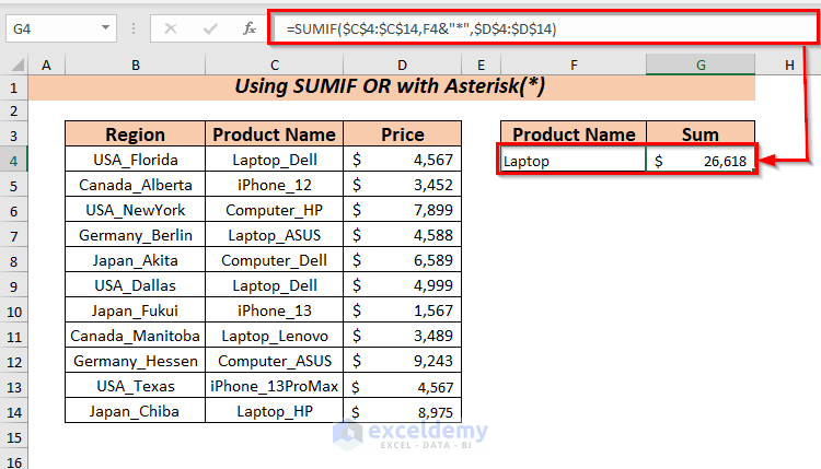
=SUMIF($C$4:$C$14,F4&"*",$D$4:$D$14)

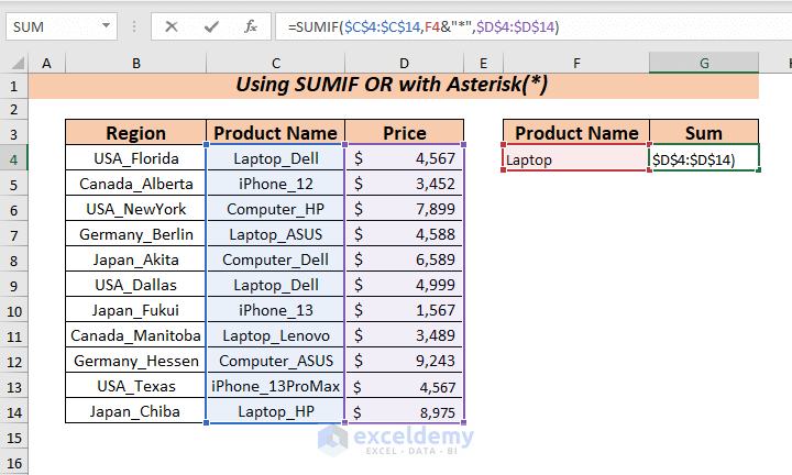Here, you can get the price for all types of laptops from the product name. I used the laptop as the criteria, and I used an asterisk (*) with the criteria. Here, an asterisk (*) will search or look up a text with a partial match. Now, in the SUMIF function, the range C4:C14 was given, and the sum_range was D4:D14. Then, it will sum the values if at least one of the partial criteria is met.

Press the ENTER key. You will see that the formula used summed the values where partial criteria are matched.

Method 7 – Using SUM & SUMIFS with OR

Steps:

Select the cell to place your resultant value.
Enter the following formula in the selected cell or into the Formula Bar:

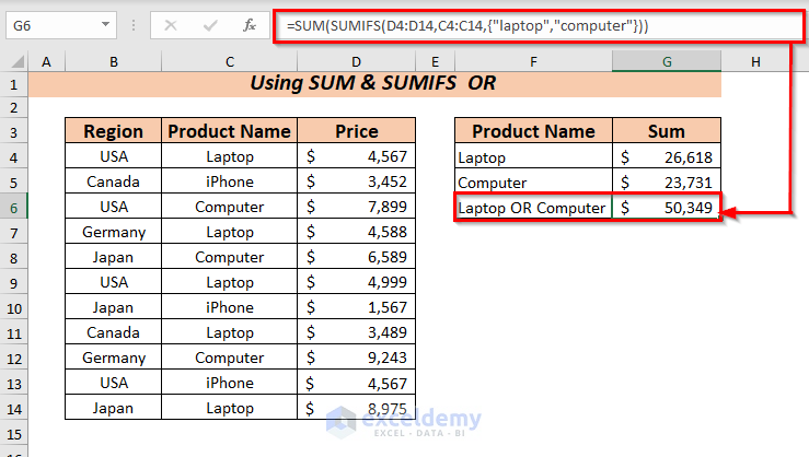
=SUM(SUMIFS(D4:D14,C4:C14,{"laptop","computer"}))

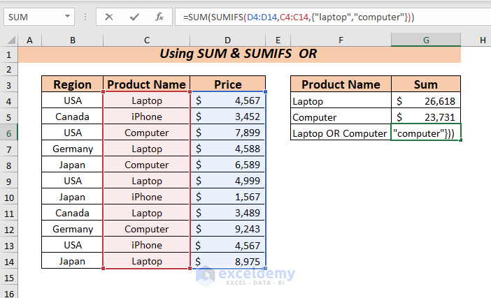Here, I want the sum of the Price using either a laptop or a computer. I used the Laptop and Computer as criteria1. Now, in the SUMIFS function, the sum_range is D4:D14, and the criteria_range1 is C4:C14. Then, the SUM function will sum the values if at least one of the criteria is met.

Press the ENTER key. You will see that the formula used summed the values where the criteria matched.

Method 8 – Using SUM & SUMIFS on Column

Steps:

Select the cell where you want to place your result.
Enter the following formula:

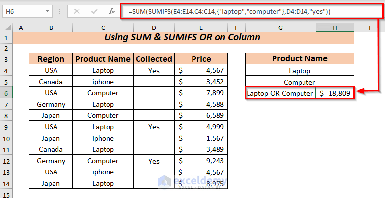
=SUM(SUMIFS(E4:E14,C4:C14,{"laptop","computer"},D4:D14,"yes"))

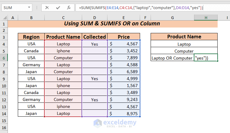Here, I used Laptop and Computer as criteria from a different column. In the SUMIFS function, take sum_range D4:D14 and criteria_range1 given the range C4:C14. In the criteria1 field, laptops and computers were used as wildcards. Then, in criteria_range2, given the range D4:D14, select the critera2 for Yes from the Collected column. Then, the SUM function will sum the values if at least one of the criteria is met.

Press the ENTER key. You will see that the used formula summed the values where different column values met at least one of the criteria.

Method 9 – Using SUM & SUMIFS with Wildcards

Steps:

Select the cell where you want to place your resultant value.
Enter the following formula:

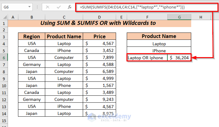
=SUM(SUMIFS(D4:D14,C4:C14,{"*laptop*","*iphone*"}))

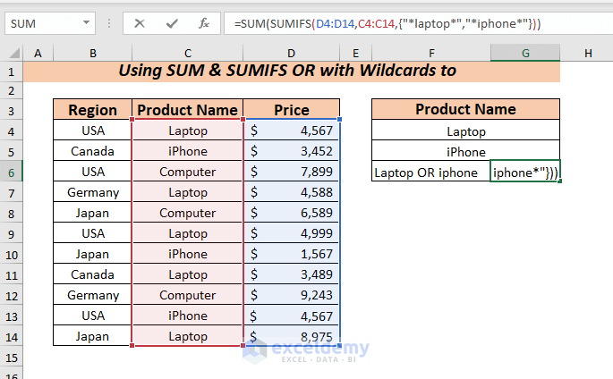Here, I wanted to sum up the price for a laptop or iPhone using the product name. So that. I used the Laptop and iPhone as criteria1 with the wildcards asterisk (*). In the SUMIFS function, the sum_range D4:D14 is given to extract the price for the given criteria_range1 C4:C14. Then, the SUM function will sum the values if at least one of the criteria is fully/ partially met.

Press the ENTER key. You will see that the used formula summed the values where partial or full criteria are matched.

Method 10 – Using SUM & SUMIFS with Multiple Criteria

Steps:

Select the cell to place your resultant value.
Enter the following formula in the selected cell or into the Formula Bar:

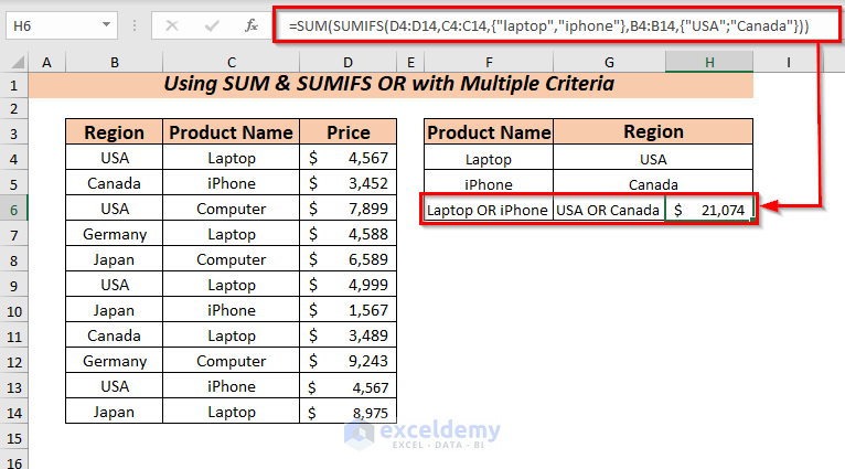
=SUM(SUMIFS(D4:D14,C4:C14,{"laptop","iphone"},B4:B14,{"USA";"Canada"}))

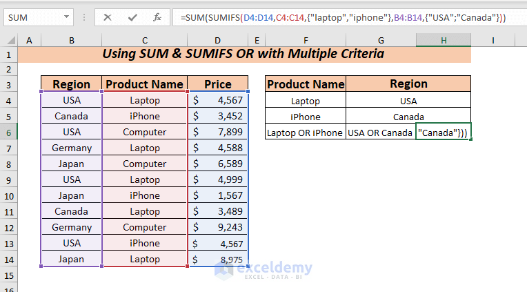Here, I used Laptop and iPhone from Product Name, the USA, and Canada from Region as criteria from a different column. Now, in the SUMIFS function, take sum_range D4:D14, and in criteria_range1, select the range C4:C14 where criteria1 used Laptop and iPhone.

Then, in criteria_range2, we have given the range B4:B14 and selected the USA and Canada as critera2. Then, the SUM function will sum the values if at least one of the criteria is met.

Here, I used a single-column array for criteria1 and the semi-colons in the second array constant for criteria2 because the latter represents a vertical array. It works for the Excel “pairs” elements in the two array constants and returns a two-dimensional array of results.