One of the most important features of Excel is to collect and contain data from various places into a single cell. In other words, to concatenate. Today I will be showing how you can concatenate the values from two or more cells in Excel.
Download Practice Workbook
Download this practice workbook to exercise while you are reading this article.
5 Simple Methods to Concatenate in Excel
In the following, I have shared 5 simple methods to Concatenate in Excel.
Here we’ve got a data set with the Employee IDs, Employee Names, and Salaries of some employees of a company named Sunflower Group. Our objective today is to concatenate all the information into a single cell called Merged Information.

1. Using Ampersand (&) Symbol
We can use the Ampersand (&) symbol to concatenate all the information into a single cell. Follow the steps below-
Steps:
- First, choose a cell (E5) and apply the below formula down-
=B5&", "&C5&", "&D5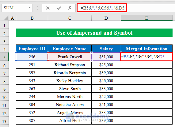
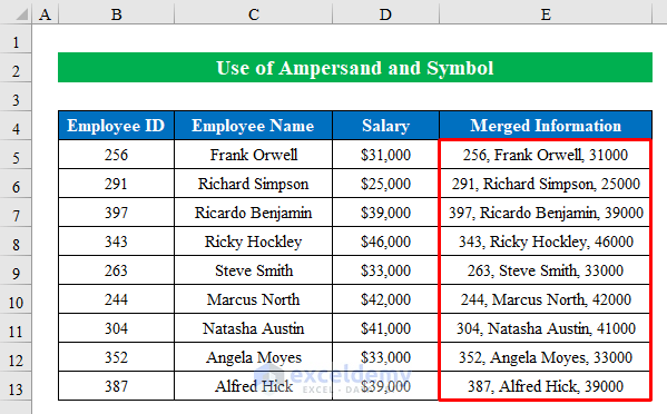
- Now press ENTER and drag the Fill Handle to fill the formula to the rest of the cells.
- In summary, we will get the information merged in a single cell. Simple isn’t it?
2. Using CONCATENATE Function
You can perform a similar task using the CONCATENATE function in Excel. You can do this by inserting all the values that you want to concatenate as the arguments of the function.
Steps:
- Start with, choosing a cell (E5) and putting the below formula down-
=CONCATENATE(B5,", ",C5,", ",D5)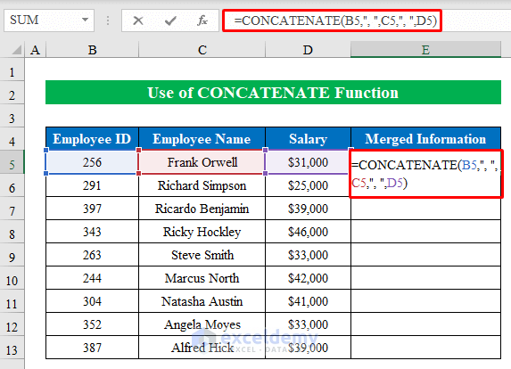
- Then drag the Fill Handle to fill the formula to the rest of the cells.
- In summary, you will get the output in your hands within a blink of an eye.

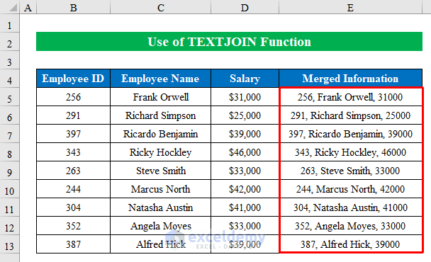
3. Excel TEXTJOIN Function to Concatenate
When you have a large range of cells to join, using the Ampersand (&) symbol or the CONCATENATE function may be a bit troublesome. In these cases, you can use the TEXTJOIN function of Excel. Follow the steps below-
Steps:
- Choose a cell (E5) and apply the formula below-
=TEXTJOIN(", ",TRUE,B5:D5)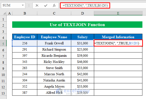
- The first argument of the TEXTJOIN function is the delimiter (By which the texts are separated). We inserted a comma (,) in this case. If you want, you can use anything else as the delimiter. It can be any string.
- The second argument indicates whether we want to ignore the empty cells within the given range or not. We set it as TRUE. That means, if there are one or more empty cells within our given range, we want to ignore those.
- The third argument is the range that we want to concatenate. It is B4:D4 for the first employee.
Read More: How to Concatenate Multiple Cells in Excel
4. Utilizing CONCAT Function to Concatenate
If you want you can also use the CONCAT function to concatenate text or numeric values in Excel.
Steps:
- Presently, choose a cell (E5) and write the below formula down-
=CONCAT(B5,", ", C5,", ",D5)Here, the CONCAT function will join values from the cell (B5:D5) into one cell.

- Gently, press ENTER and drag the “Fill Handle” down to fill the column.
- In summary, you will get the values concatenated into one single cell.

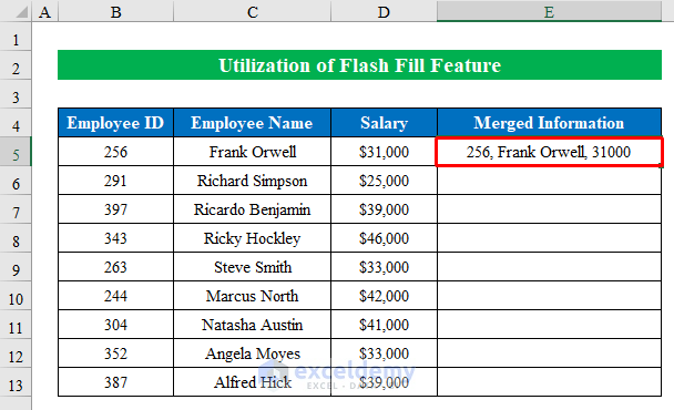
5. Using Flash Fill Feature to Concatenate
Flash fill feature is one of the most tremendous features of Excel which can help you fill multiple columns and rows with your desired values. With the flash fill feature, you can concatenate cells and fill the other rows or columns without applying formulas. Follow the instructions below-
Steps:
- Presently, in cell (E5) write your desired text or values.
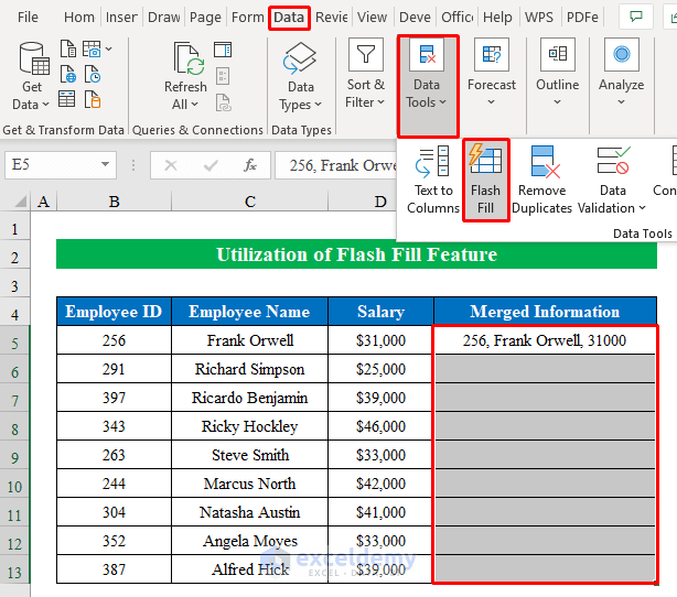
- After that, selecting cells (E5:E13) click the “Flash Fill” option from the “Data” tab.
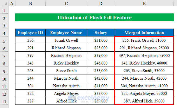
- Finally, you will get to see your desired output in the selected cells. Enjoy!
Read More: How to Concatenate Text in Excel
Conclusion
Using these methods, we can concatenate the values from two or more cells into one single cell in Excel. Do you have any questions? Feel free to ask us.
Concatenate Excel: Knowledge Hub
- Add Text to Cell Value in Excel
- Concatenate Numbers in Excel
- Concatenate Range in Excel
- Concatenate and Keep Currency Format in Excel
- Combine Two Formulas in Excel
- Concatenate with Delimiter in Excel
- Concatenate with Space in Excel
- Concatenate Apostrophe in Excel
- CONCATENATE vs CONCAT in Excel
- Excel CONCATENATE Showing Formula Not Result
- Concatenate Not Working in Excel
- Opposite of Concatenate in Excel
- Excel INDEX MATCH to Concatenate Multiple Results
- Concatenate If Cell Values Match in Excel
- Concatenate Cells with If Condition in Excel
- Concatenate with VLOOKUP in Excel
- Concatenate Decimal Places in Excel
- Add Parentheses with CONCATENATE Function in Excel
- Concatenate Different Fonts in Excel
- Combine CONCATENATE & TRANSPOSE Functions in Excel
- Add Comma in Excel
- Add Quotes in Excel
- Excel Concatenate Date
<< Go Back To Learn Excel
Get FREE Advanced Excel Exercises with Solutions!
