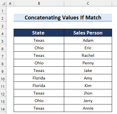
How to Concatenate If Cell Values Match in Excel (7 Easy Ways)

To demonstrate our methods we’ll use the following dataset, containing columns for State and Sales Person. We’ll concatenate the values in the Sales Person column if the States match.

Method 1 – Combining TEXTJOIN & IF Functions

We can use the TEXTJOIN function, and the IF function to concatenate if values match in Excel.

Steps:

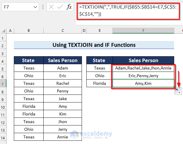
In cell F5 (the cell where we want to concatenate values), enter the following formula:

=TEXTJOIN(",",TRUE,IF($B$5:$B$14=E5,$C$5:$C$14,""))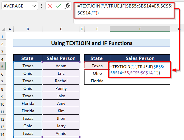

Press Enter to get the result.

How Does the Formula Work?

IF($B$5:$B$14=E5,$C$5:$C$14,””): The IF function checks if the value in cell E5 has matches in the cell range B5:B14. If the logical_test is True then the formula returns corresponding values from the cell range C5:C14.
TEXTJOIN(“,”,TRUE,IF($B$5:$B$14=E5,$C$5:$C$14,””)): The TEXTJOIN function joins the values returned by the IF function with the given delimiter of a comma (“,”).

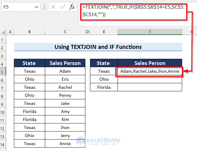
Drag the Fill Handle to copy the formula down to cell F7.

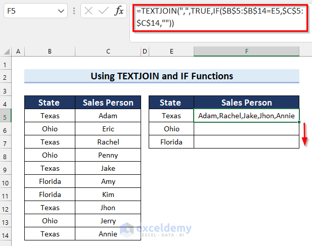
The results are as follows.

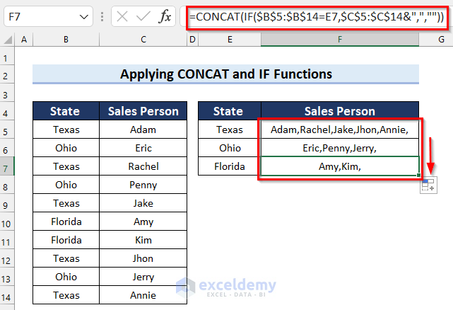
Method 2 – Using CONCAT & IF Functions

The CONCAT function joins multiple texts from different strings.

Steps:

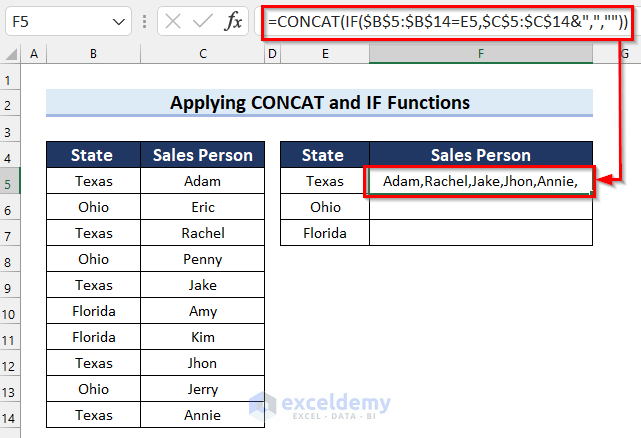
In cell F5 enter the following formula:

=CONCAT(IF($B$5:$B$14=E5,$C$5:$C$14&",",""))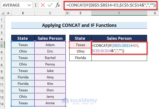

Press Enter.

How Does the Formula Work?

IF($B$5:$B$14=E5,$C$5:$C$14&”,”,””): The IF function checks if the value in cell E5 has matches in the cell range B5:B14. If the logical_test is True then the formula returns corresponding values from the cell range C5:C14 with a delimiter of a comma (“,”).
CONCAT(IF($B$5:$B$14=E5,$C$5:$C$14&”,”,””)): The CONCAT function joins the values returned by the IF function.

Drag the Fill Handle down to copy the formula.

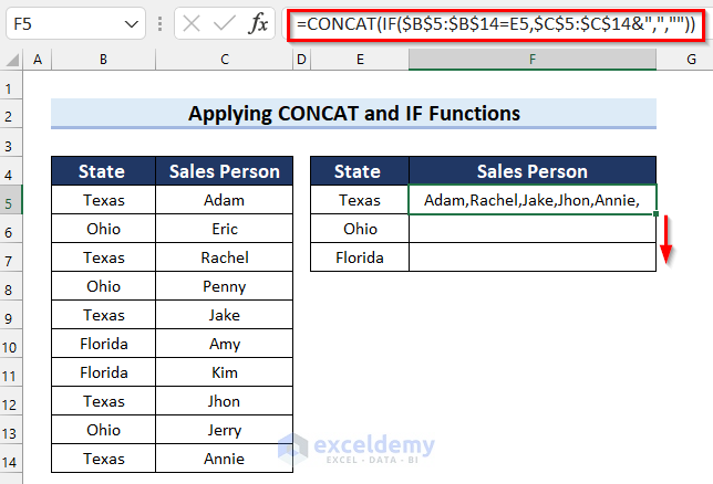
The results are as follows.

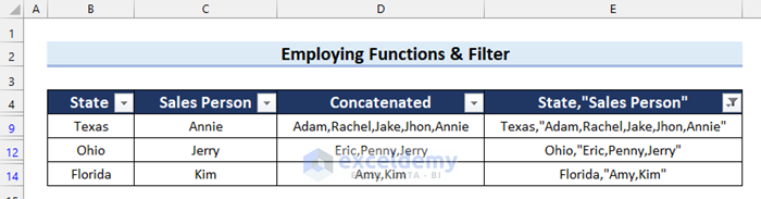
Method 3 – Using Functions & Filter

We can use functions to concatenate if the values match, then Filter the results to return the desired output. To apply this method, the values must be stored together in the same dataset.

Steps:

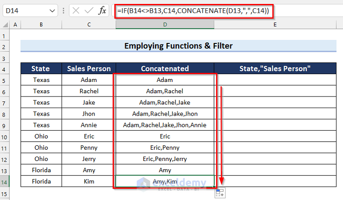
In cell D5 enter the following formula:

=IF(B5<>B4,C5,CONCATENATE(D4,",",C5))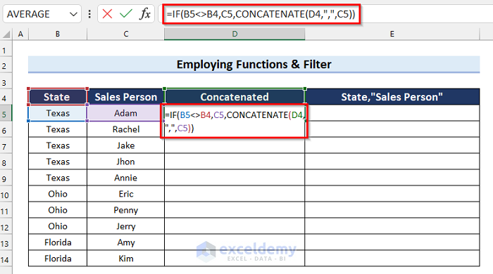

Press Enter.

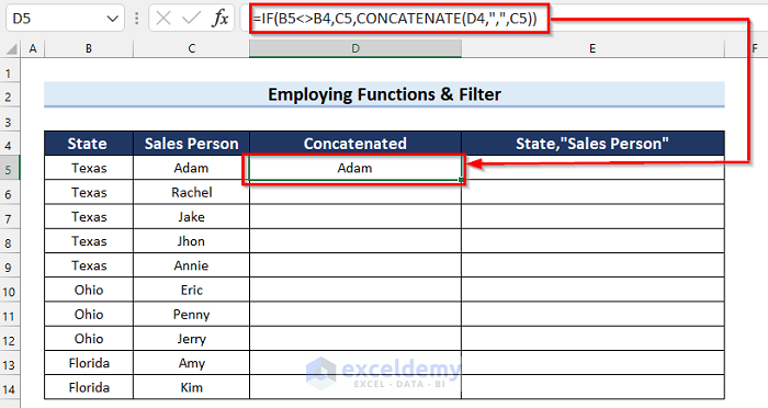
How Does the Formula Work?

IF(B5<>B4,C5,CONCATENATE(D4,”,”,C5)): The IF function checks if the value in cell B5 is not equal to the value in cell B4. If the logical_test is True then the formula will return the value in cell C5. Otherwise, it will execute the CONCATENATE function.
CONCATENATE(D4,”,”,C5): The CONCATENATE function joins the value in cell D4 with the value in cell C5 with a delimiter of a comma (“,”).

Drag the Fill Handle down to copy the formula.

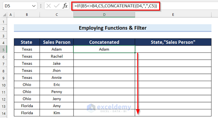
The results are as follows.

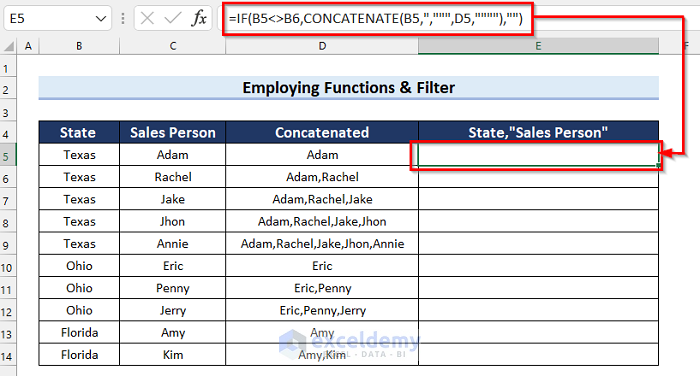
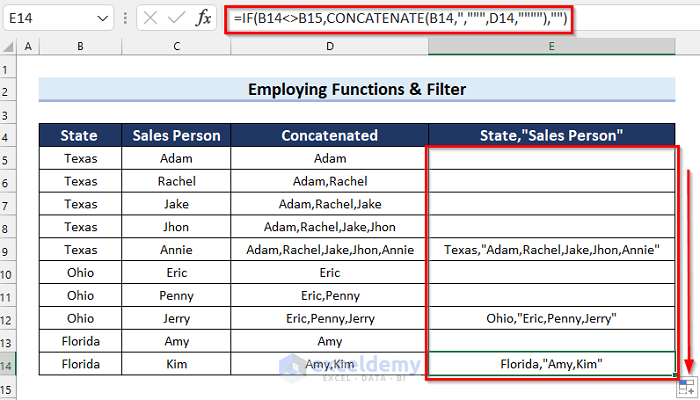
In cell E5, enter the following formula:

=IF(B5<>B6,CONCATENATE(B5,",""",D5,""""),"")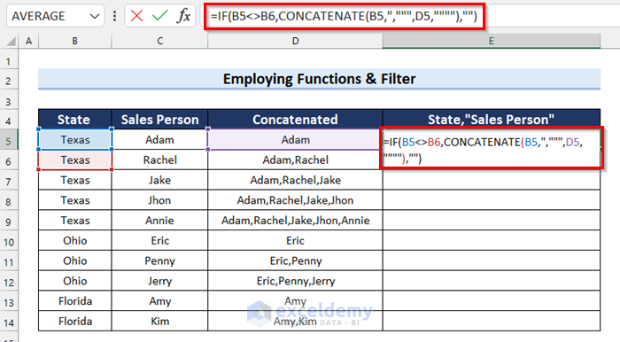

Press Enter to get the result.

How Does the Formula Work?

IF(B5<>B6,CONCATENATE(B5,”,”””,D5,””””),””): The IF function checks if the value in cell B5 is not equal to the value in cell B6. If the logical_test is True then the formula will execute the CONCATENATE function. Otherwise, it will return a blank.
CONCATENATE(B5,”,”””,D5,””””): Now, the CONCATENATE function will combine the texts.

Drag the Fill Handle down to copy the formula.

The results are as follows. Some cells are blank.

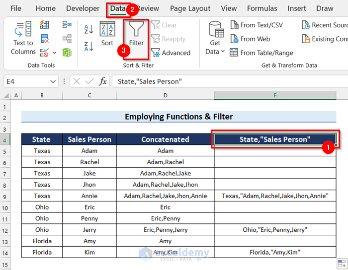
Now we’ll filter the column to get rid of the blank cells.

Select the column header where you want to apply the filter (cell E4).
Go to the Data tab.
Select Filter.

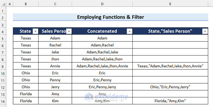
A filter is added to this dataset.

Click on the filter button on cell E4.
Uncheck the blank option.
Click OK.

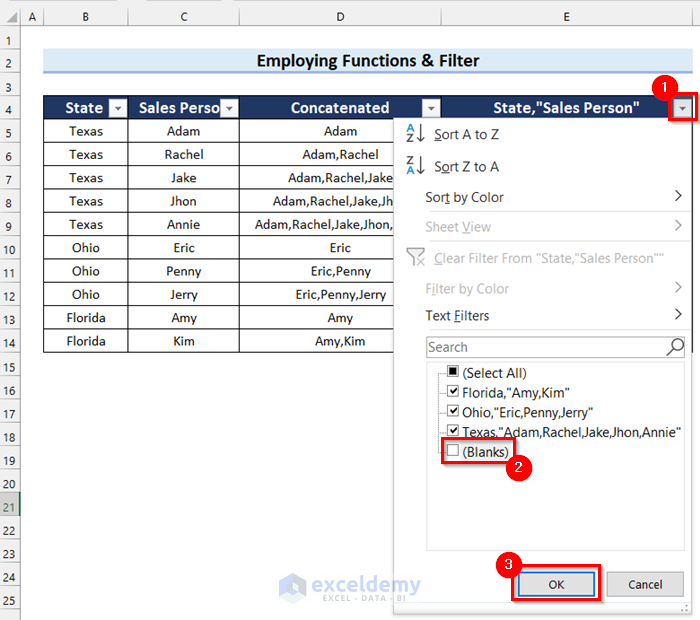
The blank cells are filtered out.

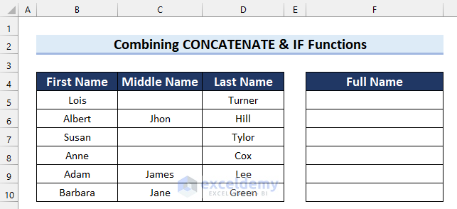
Method 4 – Combining CONCATENATE & IF Functions

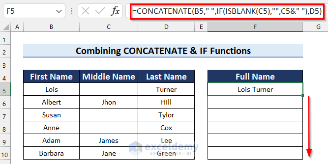
For this example, we’ll use a different dataset containing 3 columns; First Name, Middle Name, and Last Name. The Middle Name column contains some blank cells. Let’s match the blanks and then concatenate the values accordingly if a match is found or not.

Steps:

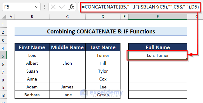
In cell F5 enter the following formula:

=CONCATENATE(B5," ",IF(ISBLANK(C5),"",C5&" "),D5)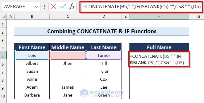

Press Enter.

How Does the Formula Work?

ISBLANK(C5): The ISBLANK function will return True if cell C5 is blank. Otherwise, it will return False.
IF(ISBLANK(C5),””,C5&” “): The IF function checks for matches and if the logical_test is True returns blank. Otherwise, it returns the value in cell C5 followed by a space.
CONCATENATE(B5,” “,IF(ISBLANK(C5),””,C5&” “),D5): The CONCATENATE function will join the resultant text.

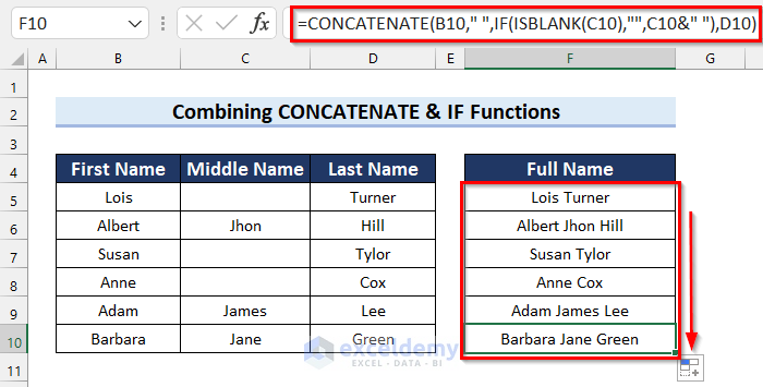
Drag the Fill Handle down to copy the formula to the other cells.

Full Names include Middle Names where those are present in column C, otherwise they don’t.

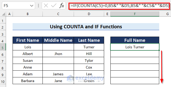
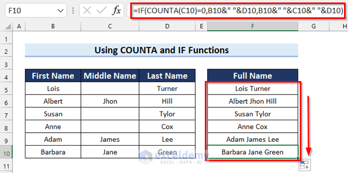
Method 5 – Using COUNTA Function

The COUNTA function counts cells containing any kind of information, and can be used to find the blank cells, then used in conjunction with the IF function to concatenate the matches accordingly.

Steps:

In cell F5 enter the following formula:

=IF(COUNTA(C5)=0,B5&" "&D5,B5&" "&C5&" "&D5)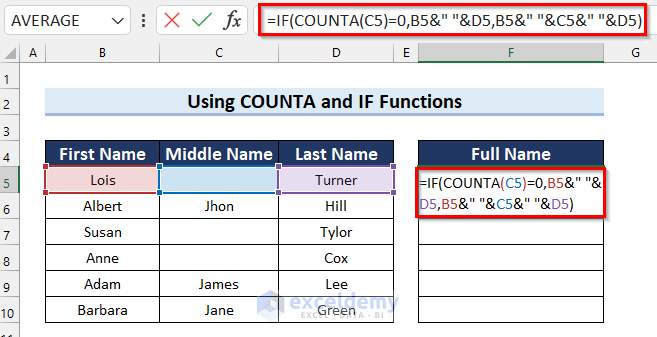

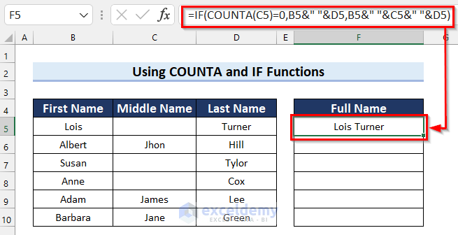
Press Enter to get the result.

How Does the Formula Work?

COUNTA(C5): The COUNTA function returns the number of cells containing any values.
IF(COUNTA(C5)=0,B5&” “&D5,B5&” “&C5&” “&D5): The IF function checks if the COUNTA function returns 0. If the logical_test is True then the formula will concatenate the values in cells B5 and D5. Otherwise, it will concatenate the values in cells B5, C5, and D5.

Drag the Fill Handle down to copy the formula.

The results are as follows.

Method 6 – Using VBA Code

The VBA macro below will concatenate cell values if they match, and return the results with the column header.

Steps:

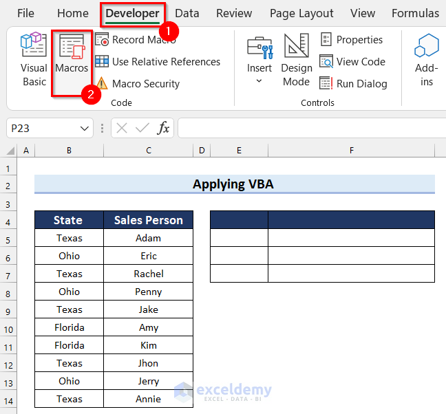
Go to the Developer tab.
Select Visual Basic.

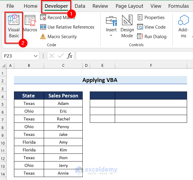
The Visual Basic Editor window will open.

Select the Insert tab.
Select Module.

A module will open.

Enter the following code in the module:

Sub Concatenate_If_Match()
    Dim t_col As New Collection
    Dim inp_table As Variant
    Dim output() As Variant
    Dim m As Long
    Dim col_no As Long
    Dim rng As Range
    inp_table = Range("B4", Cells(Rows.Count, "B").End(xlUp)).Resize(, 2)
    Set rng = Range("E4")
    On Error Resume Next
    For m = 2 To UBound(inp_table)
        t_col.Add inp_table(m, 1), TypeName(inp_table(m, 1)) & CStr(inp_table(m, 1))
    Next m
    On Error GoTo 0
    ReDim output(1 To t_col.Count + 1, 1 To 2)
    output(1, 1) = "State"
    output(1, 2) = "Sales Person"
    For m = 1 To t_col.Count
        output(m + 1, 1) = t_col(m)
        For col_no = 2 To UBound(inp_table)
            If inp_table(col_no, 1) = output(m + 1, 1) Then
                output(m + 1, 2) = output(m + 1, 2) & ", " & inp_table(col_no, 2)
            End If
        Next col_no
        output(m + 1, 2) = Mid(output(m + 1, 2), 2)
    Next m
    Set rng = rng.Resize(UBound(output, 1), UBound(output, 2))
    rng.NumberFormat = "@"
    rng = output
    rng.EntireColumn.AutoFit
End Sub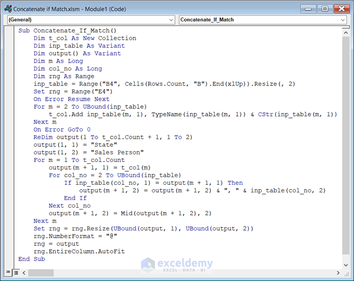

How Does the Code Work?

We create a Sub Procedure named Concatenate_If_Match.
We declare the variables.
We use a Set Statement to set where we want the output.
We use a For Next Loop to go through the input table.
We use the ReDim Statement to size the declared array.
We use another For Next Loop to go through the columns.
We use an IF Statement to check for a match.
We end the Sub Procedure.

Save the code and go back to the worksheet.
Go to the Developer tab.
Select Macros.

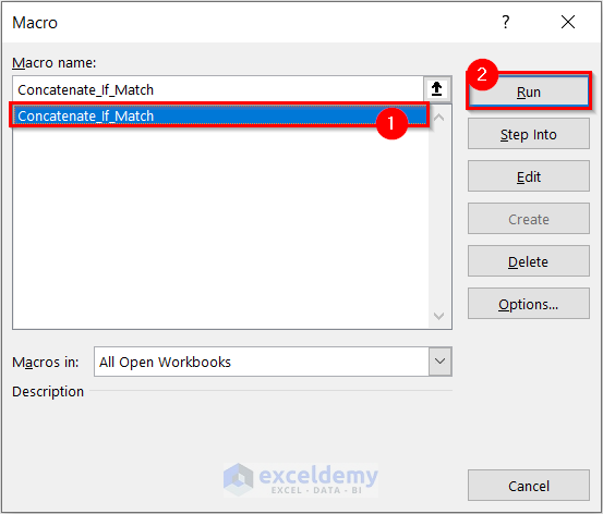
The Macro dialog box will appear.

Select Concatenate_If_Match as Macro Name.
Click Run.

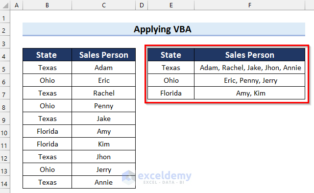
The desired output is returned.

Method 7 – Using a User Defined Function

A user defined function is a function defined by the user for a specific task, and created by writing a VBA code. Let’s create a User defined function to concatenate if cell values match.

Steps:

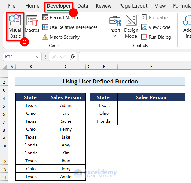
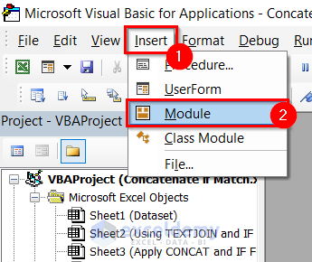
Go to the Developer tab.
Select Visual Basic.

The Visual Basic Editor window will open.

Go to the Insert tab.
Select the Module.

A module will open.

Enter the following code in the module:

Function CONCATENATE_IF(criteria_range As Range, criteria As Variant, _
concatenate_range As Range, Optional Delimiter As String = ",") As Variant
Dim Results As String
On Error Resume Next
If criteria_range.Count <> concatenate_range.Count Then
    CONCATENATE_IF = CVErr(xlErrRef)
    Exit Function
End If
For J = 1 To criteria_range.Count
    If criteria_range.Cells(J).Value = criteria Then
        Results = Results & Delimiter & concatenate_range.Cells(J).Value
    End If
Next J
If Results <> "" Then
    Results = VBA.Mid(Results, VBA.Len(Delimiter) + 1)
End If
CONCATENATE_IF = Results
Exit Function
End Function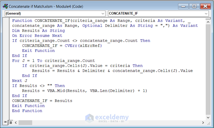

How Does the Code Work?

We create a Function named CONCATENATE_IF.
We declare the variables for the function.
We use an If Statement to check for a match.
We use the CVErr function to return a user defined error.
We use a For Next Loop to go through the whole range.
We use another If Statement to find a match and then return results accordingly.
We end the Sub Procedure.

Save the code and go back to the worksheet.
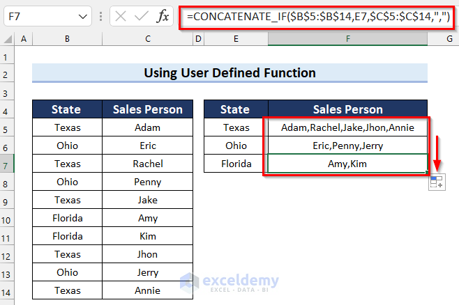
In cell F5 enter the following formula:

=CONCATENATE_IF($B$5:$B$14,E5,$C$5:$C$14,",")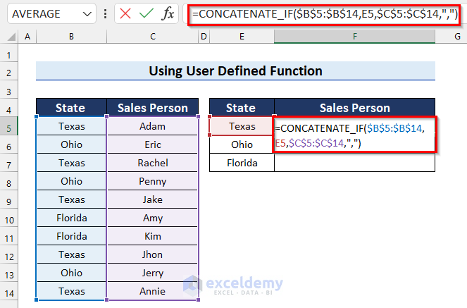

Press Enter to get the result.

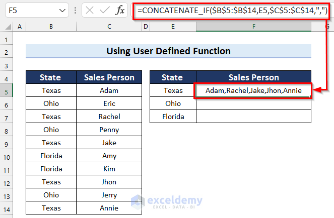
Here, we selected cell range B5:B14 as criteria_range, cell E5 as criteria, cell range C5:C14 as concatenate_range, and “,” as Delimiter. The formula will concatenate the values from the concatenate_range if the criteria match the criteria_range.

Drag the Fill Handle down to copy the formula.

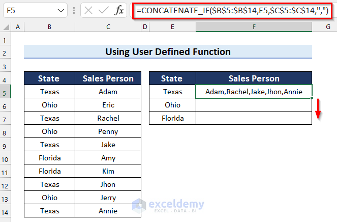
The desired output is returned.

Things to Remember

If you use VBA in your Excel workbook then you must save the Excel file as Excel Macro-Enabled Workbook. Otherwise, the VBA code will not work.

Download Practice Workbook

Concatenating Values If Match.xlsm

Get FREE Advanced Excel Exercises with Solutions!

How to Concatenate If Cell Values Match in Excel (7 Easy Ways)

Method 1 – Combining TEXTJOIN & IF Functions

Method 2 – Using CONCAT & IF Functions

Method 3 – Using Functions & Filter

Method 4 – Combining CONCATENATE & IF Functions

Method 5 – Using COUNTA Function

Method 6 – Using VBA Code

Method 7 – Using a User Defined Function

Things to Remember

Related Articles

Leave a reply Cancel reply