Introduction to the CONCATENATE Function
- Syntax:
=CONCATENATE(text1,[text2],...)- Argument:
text1– the first text, number, or array you want to join.
[text2],…– More text, numbers, or arrays that you want to join.
- Function:
Returns the concatenated array combining all the values or arrays.
- Example:
Suppose we have a dataset containing 4 text values in cell range C4:F4. We want to join these text values using the CONCATENATE function.
Steps:
- Select Cell C5 and insert the following formula.
=CONCATENATE(C4:F4)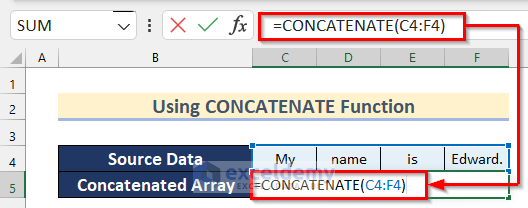
- Select the whole formula and press F9 on your keyboard to convert the formula into values.
![]()
- Remove the Curly Brackets ({}) from the formula like the image shown below.
![]()
- Press Enter, and you will get your desired Concatenated Array.
![]()
Introduction to the TRANSPOSE Function
- Syntax:
=TRANSPOSE (array)- Argument:
array– the cell range or array you want to transpose.
- Function:
Converts a vertical range or array into horizontal and vice versa.
- Example:
Suppose we have text values in the vertical cell range B5:B12. To convert the range into a horizontal one, insert the following formula in Cell D5 and press Enter:
=TRANSPOSE(B5:B12)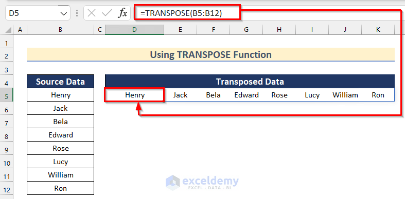
3 Examples of Using CONCATENATE and TRANSPOSE Functions Together in Excel
Example 1 – Combining Text
We have some text values in cell range B5:B11. We will join and transpose these values.
![]()
Steps:
- Select Cell D5 and insert the following formula.
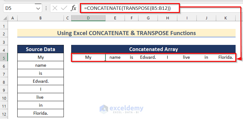
=CONCATENATE(TRANSPOSE(B5:B12))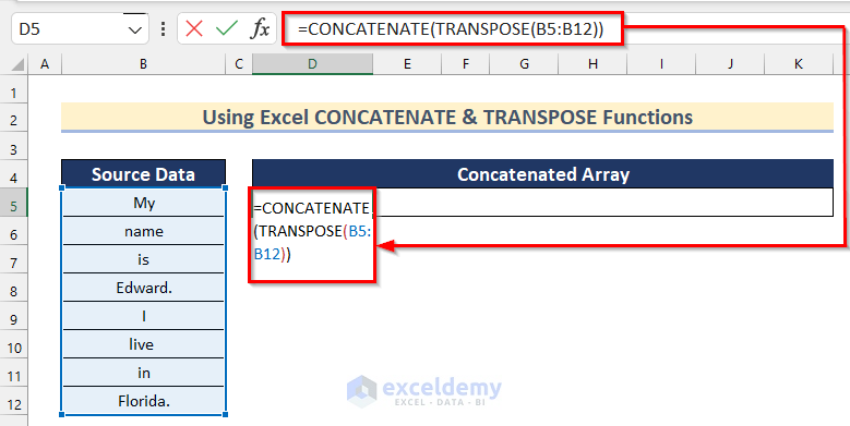
- Press Enter and get your desired Concatenated Array.
How Does the Formula Work?
- The TRANSPOSE function converts the vertical cell range B5:B12 into a horizontal one.
- The CONCATENATE function joins the values in that cell range.
Example 2 – Apply CONCATENATE and TRANSPOSE Functions with Commas and Spaces
We have the Names of some students. We will add a comma and space between each name and list them.
![]()
Steps:
- Insert the following formula in Cell D5.
=CONCATENATE(TRANSPOSE(B5:B12&", "))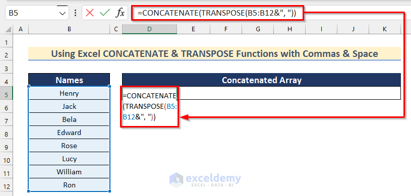
- Press Enter and get your desired Concatenated Array.
![]()
How Does the Formula Work?
- The TRANSPOSE function converts the vertical cell range B5:B12 into a horizontal one and adds a comma and space using the Ampersand Operator (&).
- The CONCATENATE function joins the values in that cell range.
Read More: How to Concatenate Cells with If Condition in Excel
Example 3 – Add Characters Along Values
In the last method, we will show you how you can add characters along with CONCATENATE & TRANSPOSE functions in a merged cell.
![]()
Steps:
- Insert the following formula in the merged cell.
=TRANSPOSE(B5:B12&" ")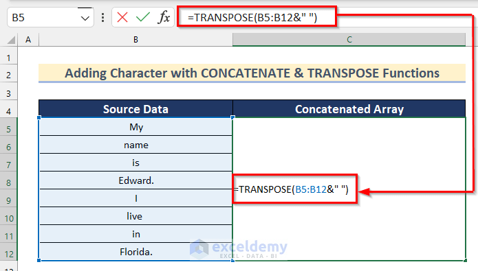
- Select the whole formula and press F9 on your keyboard to convert the formula into values like this.
![]()
- Add the CONCATENATE function at the beginning and remove the Curly Brackets ({}) as follows.
![]()
- Press Enter and you will see the required output.
![]()
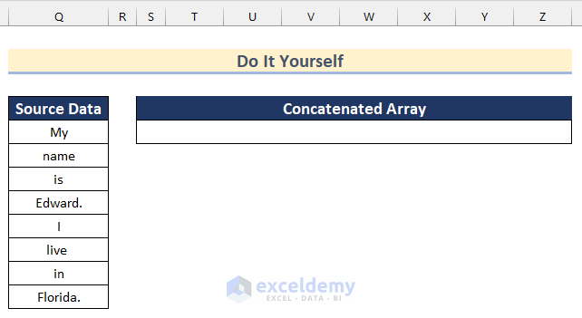
Practice Section
In the article, you will find an Excel workbook like the image given below to practice on your own.
Download the Practice Workbook
Related Articles
- How to Concatenate If Cell Values Match in Excel
- How to Concatenate with VLOOKUP in Excel
- How to Concatenate Email Addresses in Excel
- How to Concatenate Decimal Places in Excel
- How to Concatenate Different Fonts in Excel

