While working in Microsoft Excel we might need to concatenate different multiple results from a particular dataset. In this article, we will demonstrate 2 easy steps of how to use INDEX MATCH to concatenate multiple results. To clarify the steps to you we will use a unique dataset with different types of formulas.
Introduction to the Excel INDEX Function
-
Description
The INDEX function gives a value or reference of a value for a particular table or range in return.
-
Syntax
INDEX(array, row_num, [column_num], [area_num])
-
Arguments
| ARGUMENTS | REQUIREMENT | EXPLANATION |
|---|---|---|
| array | Required | Indicates cell range or an array constant. |
| row_num | Required | The position of the row from which a reference will return. |
| [column_num] | Optional | The position of the column from which a reference will return. |
| [area_num] | Optional | The used range in reference. |
Introduction to the Excel MATCH Function
-
Description
In Microsoft Excel, the MATCH function finds specific values in a range of cells.
-
Syntax
MATCH(lookup_value, lookup_array, [match_type])
-
Arguments
| ARGUMENTS | REQUIREMENT | EXPLANATION |
|---|---|---|
| lookup_value | Required | Indicates the value that will be searched in a range. |
| lookup_array | Required | The range where the value will be searched |
| [match_type] | Optional | Used to indicate the match type for the function. Generally, it’s a numerical value. Three types of match type can be applied:
0 to find an exact match. 1 to find the largest value that is less than or equal to search value. -1 to find the smallest value that is greater than or equal to search value. |
Excel INDEX MATCH to Concatenate Multiple Results: 2 Easy Steps
Using excel INDEX MATCH functions to concatenate multiple results is one single process. But to make you understand better we will explain the method in two steps.
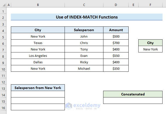
Dataset Introduction of INDEX MATCH to Concatenate Multiple Results
We have a dataset (B4:B10) for salespersons with their functioning cities and sales amount. We are going to apply INDEX MATCH functions to concatenate the name of the salespersons working in the same city.
Step-1: Use INDEX MATCH Functions to Extract Values with the Same Index for Multiple Results
In the first step we will extract the names of the salespersons who are working in New York in cells (C14:C16). Now, let’s go through the following steps to perform this action. To execute this method we will use some more functions besides the INDEX MATCH functions. The functions are-
- SMALL Function: The SMALL function returns the smallest value from an array in a specific position.
- IF Function: The IF function is used to compare between two values and returns any specific result.
- ISNUMBER Function: The ISNUMBER function inspects whether a cell value is a number or not.
Let’s see how these functions work combinedly:
- Firstly, select cell B14.
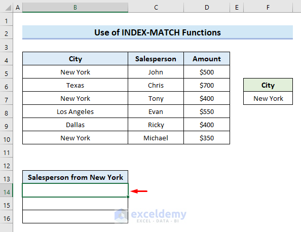
- Secondly, insert the following formula in that cell:
=INDEX($C$5:$C$10,SMALL(IF(ISNUMBER(MATCH($B$5:$B$10,$F$7,0)),MATCH(ROW($B$5:$B$10), ROW($B$5:$B$10)),""),ROWS($A$1:A1)))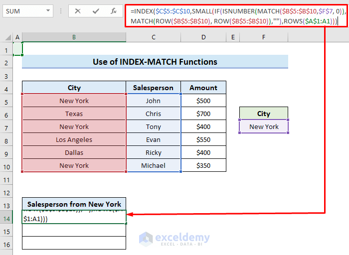
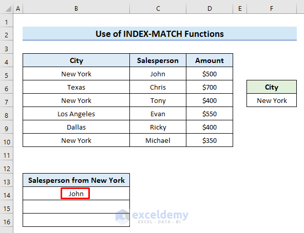
- Then, press Enter. So, it returns the name of the first salesperson working in New York in cell B14.
- Thirdly, select cell B14. Move the mouse cursor to the bottom right corner of the selected cell so that it turns into a plus (+) sign like the following image.
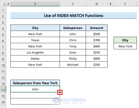
- After that, click on the plus (+) sign and drag the Fill Handle down to cell B16 to copy the formula of cell B14 in other cells. We can also double-click on the plus (+) sign to get the same result.
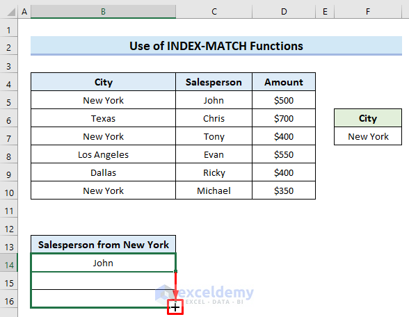
- Finally, we can see all the names of salespersons working in New York in cells (B14:B16).

🔎 How Does the Formula Work?
- ROWS($A$1:A1): This part takes cell A1 as a reference.
- ROW($B$5:$B$10)): Selects rows B5 to B10.
- MATCH(ROW($B$5:$B$10), ROW($B$5:$B$10)),””): This part searches in range (B5:B10) and returns the values that match exactly.
- (MATCH($B$5:$B$10,$F$7, 0)): This part searches in range (B5:B10) and finds the values that match with the value of cell F7.
- ISNUMBER(MATCH($B$5:$B$10,$F$7, 0): This checks if the matching values in the range (B5:B10) are numbers or not.
- IF(ISNUMBER(MATCH($B$5:$B$10,$F$7, 0)): IF formula checks the values from range (B5:B10) and returns if it gets any matching values.
- SMALL(IF(ISNUMBER(MATCH($B$5:$B$10,$F$7, 0)),MATCH(ROW($B$5:$B$10), ROW($B$5:$B$10)),””),ROWS($A$1:A1)): Returns the smallest matching value for any specific array.
- INDEX($C$5:$C$10,SMALL(IF(ISNUMBER(MATCH($B$5:$B$10,$F$7, 0)),MATCH(ROW($B$5:$B$10), ROW($B$5:$B$10)),””),ROWS($A$1:A1))): This formula looks for the matching values in the array (C5:C10) and returns in cell (B14:B16).
Read More: How to Concatenate Cells with If Condition in Excel
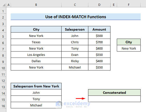
Step-2: Apply TEXTJOIN Formula to Concatenate Multiple Results
In the second step we will concatenate the results that we got by applying the INDEX MATCH functions in the previous step. To concatenate the results we will use the TEXTJOIN function. In excel, the TEXTJOIN function concatenates multiple strings in a single cell and uses a delimiter to separate the values from one another. In the following dataset, we will concatenate the results of the cells (B14:B16) in cell D15. So, to perform this action we will follow the simple steps given below.
- First, select cell D15.
- Next, insert the following formula in that cell:
=TEXTJOIN("|",TRUE,B14:B16)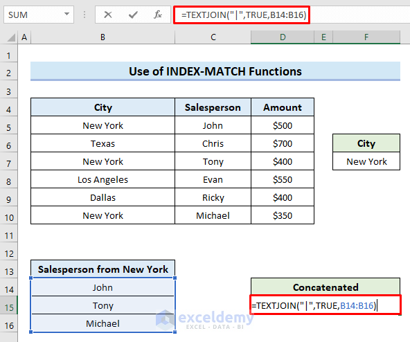
- After that, press Enter.
- Finally, we get the results of cells (B14:B16) concatenated in cell D15.

Download Practice Workbook
You can download the practice workbook from here.
Conclusion
In conclusion, this article will show you how to use index match to concatenate multiple results in excel. So, to put your skills to the test, use the practice worksheet that comes with this article. Please leave a comment below if you have any questions. Our team will try to reply to you as soon as possible. In the future, keep an eye out for more innovative Microsoft Excel solutions.
Related Articles
- How to Concatenate Arrays in Excel
- How to Concatenate If Cell Values Match in Excel
- How to Concatenate with VLOOKUP in Excel
- How to Concatenate Email Addresses in Excel
- How to Concatenate Decimal Places in Excel
- How to Add Parentheses with CONCATENATE Function in Excel
- How to Concatenate Different Fonts in Excel
- Combine CONCATENATE & TRANSPOSE Functions in Excel


Dear Sir,
I need excel formula whenever I has used INDEX formula with CONCATENATE for exciple
cell A5 value (pilus, subtract, multiplication & devidation) with cell A7 value i need total sum value in cell A5 (1+2=3)
Your help needed here.
BR,
Ahsan
Greetings Ahsan Ahmed,
It’s not clear why you want to use the INDEX-MATCH formula in the first place. However, if I assume you want to use the INDEX-MATCH formula for fetching some matching values, then you want to Add, Subtract, Multiply, or Divide them. You can use the below formula to return the matched values. And afterwards, you can execute any Arithmetic Operations you want.
=IFERROR(INDEX($D4:$D$9,IF(ISNUMBER(MATCH($B$4:$B$9,$F$6,0)),MATCH(ROW($B$4:$B$9),ROW($B$4:$B$9)),""),ROWS($A$1:A1)),"")Hope, the formula may satisfy your cravings.
Regards
Maruf Islam (Exceldemy Team)
Thats fungtion is error #VALUE!
Hello EDI,
the INDEX-MATCH formula can return a #VALUE! error under certain circumstances.
1. The MATCH function within the INDEX-MATCH formula couldn’t find a match for the lookup value in the specified array or range.
2. The INDEX function is expecting a numeric value as a result, but the matched value is non-numeric.
3. Incorrect arguments or ranges.
If you elaborate the problem you’re facing, then it will be easy to provide solution. Let us know if you face any difficulties.
Regards
Rafiul Hasan
Team ExcelDemy