Method 1 – Split Text into Multiple Cells with Formula
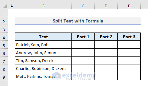
In the following table, Column B contains five distinct cells, each of which contains three names separated by a common delimiter ‘Comma’ (,). The names will be entered into three separate columns with headers Part 1, Part 2, and Part 3.
Step 1:
Select Cell C5 and enter the below formula.
=TRIM(MID(SUBSTITUTE($B5,",",REPT(" ",999)),COLUMNS($A:A)*999-998,999))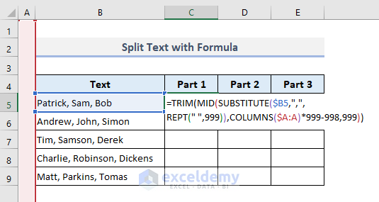
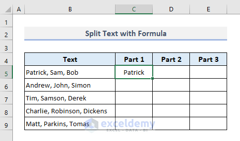
Step 2:
Press Enter and the first name will be split from the names in Cell B5.
How Does the Formula Work?
- REPT(” “,999): Here the REPT function repeats the character ‘space’ 999 times inside the SUBSTITUTE function.
- SUBSTITUTE($B5,”,”,REPT(” “,999)): The SUBSTITUTE function substitutes commas with the repeated spaces in the previous step. The formula returns the name Patrick with spaces.
- COLUMNS($A:A)*999-998: The COLUMNS function here counts the number of columns and assigns the resultant value as the start_num for the MID function.
- MID(SUBSTITUTE($B5,”,”,REPT(” “,999)),COLUMNS($A:A)*999-998,999): The MID function returns the names ‘Patrick’ with 999 characters in total.
- The TRIM function removes all unnecessary spaces from the text string found by the MID function and returns only the name ‘Patrick’.
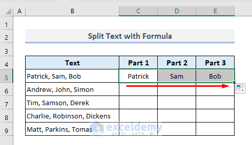
Step 3:
From Cell C5, use the Fill Handle to drag the formula to the right until all three names have been separated.
Step 4:
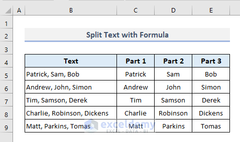
Drag the Fill Handle down to autofill the rest of the cells ranging from C6 to E9.
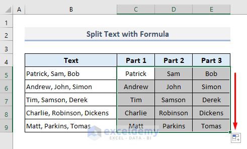
All the names from the groups of names in Column B have been separated.
Read More: How to Concatenate with Delimiter in Excel
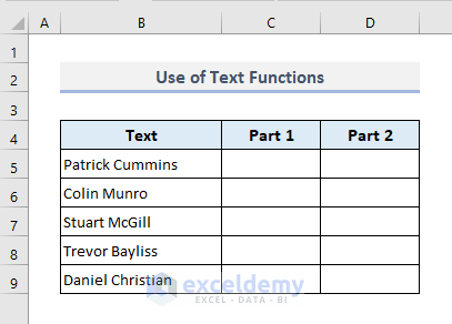
Method 2 – Opposite of Concatenate: Use of Text Functions to Split into Multiple Cells
Step 1:
Select the first output Cell C5 and enter the below formula.
=LEFT(B5,FIND(" ",B5)-1)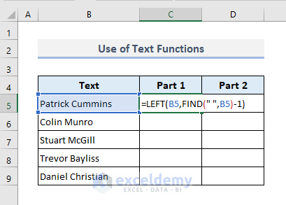
Step 2:
Press Enter and use Fill Handle to autofill the rest of the cells in Column C.

Step 3:
In Cell D5, enter the following formula.
=RIGHT(B5,LEN(B5)-FIND(" ",B5))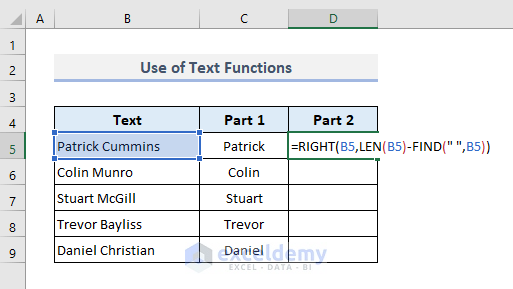
The surnames are returned in the second column.

How Does the Formula Work?
- In this formula, the LEN function returns the total number of characters available in Cell B5 and that is 15.
- The FIND function returns the position of the space found in that text and returns 8.
- The arithmetic difference between the two previous numerical values assigns the number of characters for the RIGHT function.
- The RIGHT function extracts 15-8=7 characters from the right and returns the name ‘Cummins’.
Read More: How to Concatenate with Space in Excel
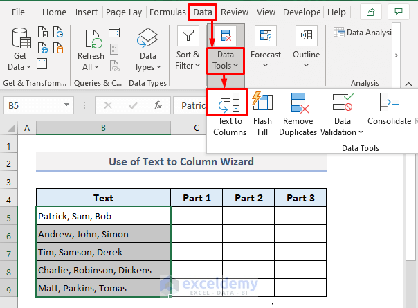
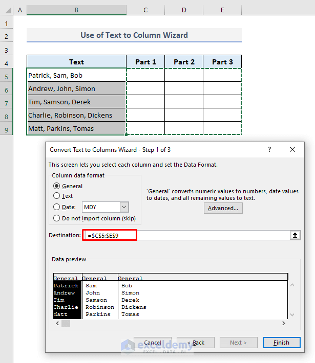
Method 3 – Use Text to Column Wizard to Reverse Concatenate in Excel
Step 1:
Select the range of cells (B5:B9) containing all text data that have to be split.
Under the Data tab, select the Text to Columns option from the Data Tools.
A dialogue box will open.
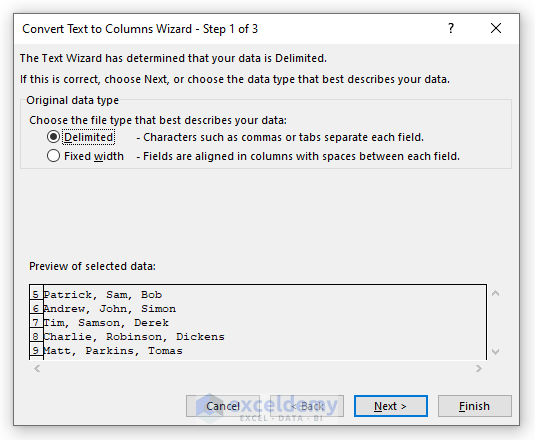
Step 2:
Choose the radio button ‘Delimited’ as the original data type.
Press Next.
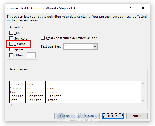
Step 3:
From the Delimiters options, mark the Comma box only and leave the other options unmarked.
Press Next.
Step 4:
Retain General as the Column Data Format.
Enable editing in the Destination box and select the output cells ranging from C5 to E9.
Press Finish.
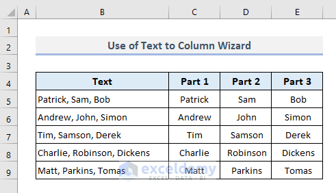
All the names in the selected output range of cells have been separated.
Read More: How to Concatenate Apostrophe in Excel
Method 4 – Apply the Flash Fill Method to Work as Opposite of the Concatenate
Step 1:
Select Cell C5 and type Patrick manually.

Step 2:
Use the Fill Handle to drag down to the last Cell C9.
Click on the options and select Flash Fill now.
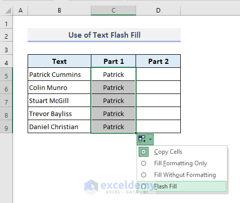
All the first names have been separated and extracted to Column C.

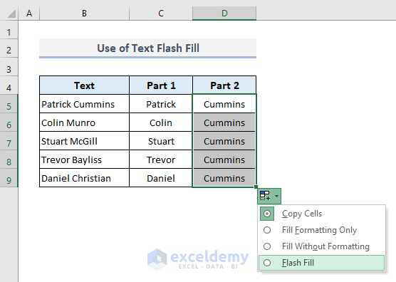
Step 3:
Do the same for the surnames under the Part 2 header.

Read More: How to Bold Text in Concatenate Formula in Excel
Download Practice Workbook
Further Readings
- How to Concatenate Cells but Keep Text Formatting in Excel
- CONCATENATE vs CONCAT in Excel
- Concatenate Not Working in Excel


I am using a form on my website to collect CVs and the excel output is like below:
Degree | College Name | Discipline | Year of Graduation | GPA
Masters | Oxford | Mathematics | 2020 | 88
Bachelors | Cambridge | Chemistry | 2016 | 76
Diploma | George’s School | Arts | 2012 | 94
All the above lies in a single cell in excel / CSV file.
Can anybody please help me how I can rearrange all this into an excel table with each cell showing part of the entries.
I do not want to use the “Text to Columns” method, because there are several such tables created and they have to be done automatically by a formula.
I appreciate your solutions.
best regards,
Nasser
Hello Nasser Enami, you can follow this article to solve your problem.
https://www.exceldemy.com/separate-address-in-excel-with-comma
In this article, you will find how to separate an address into a city, state, and zip code using an Excel formula. You can modify this file for your purpose. In your dataset the separator is “|” and you have to use 3 separators. Modify this worksheet as shown in the screenshot below-
Let us know the outcome in the reply. Thank you!
We shall try to help. Thanks.