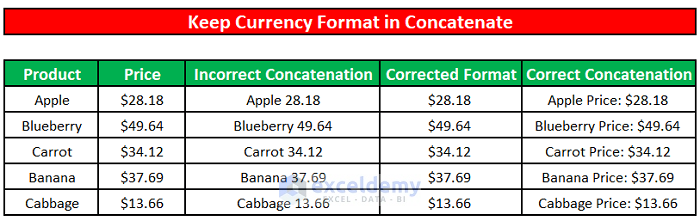
While concatenating two or more pieces of text in Excel, different number formats like currency, decimal format, and percentage format are removed and displays as general number format in the concatenated text. We can fix this by using different concatenation formulas.
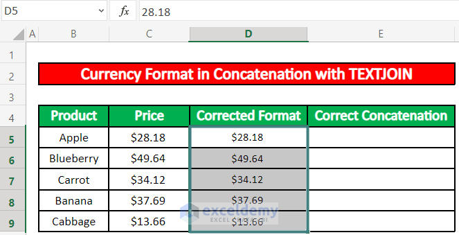
The sample dataset contains information about different fruits and their prices. We have concatenated the name of each fruit with its associated price. The prices of the fruits were output in general number format in the Incorrect Concatenation column.
Method 1 – Apply Format Cell Option and Keep Currency Format
To keep the currency format in concatenation, we can change the format of the cells.
Step 1:
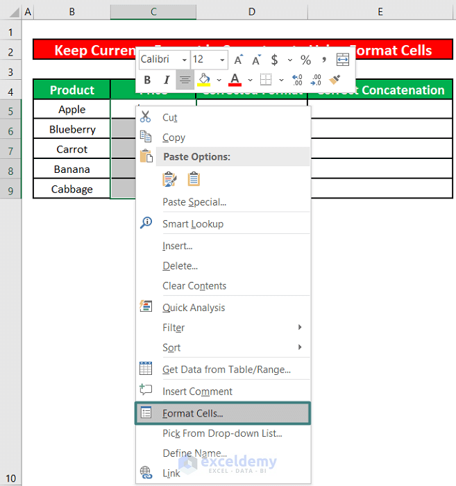
- Select all the cells in the Price column except for the column header and right-click on any of the selected cells.
- Click on Format Cells in the context menu.
Step 2:
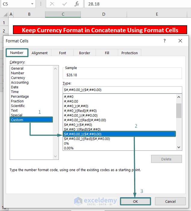
- Click on the Number tab, click on Custom from the Category.
- Select the $#,##0.00_);($#,##0.00) format from the Type of number formats section.
Step 3:
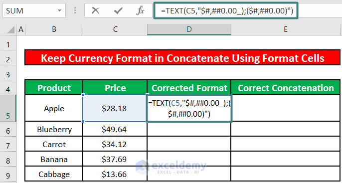
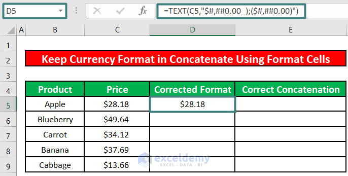
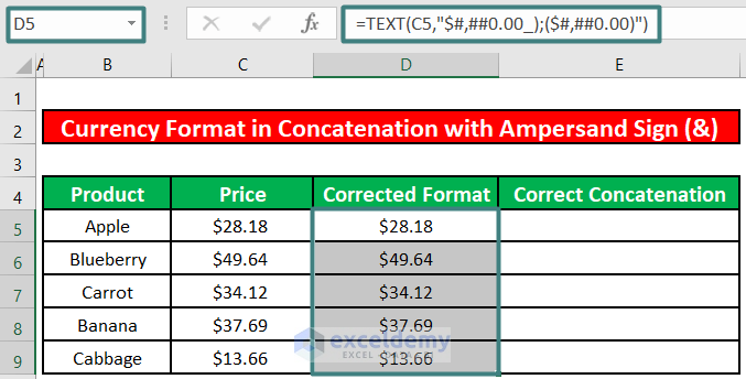
- Enter the following formula in cell D5.
=TEXT(C5,"$#,##0.00_);($#,##0.00)")Formula Breakdown:
The TEXT formula will format the price (C5) using the $#,##0.00_);($#,##0.00) format.
- Press ENTER.
- The price in cell C5 will be formatted as currency in cell D5.
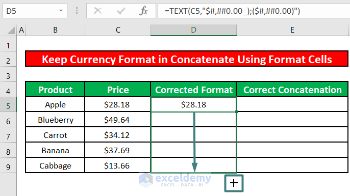
- Use the fill handle tool to apply the formula to the rest of the cells.
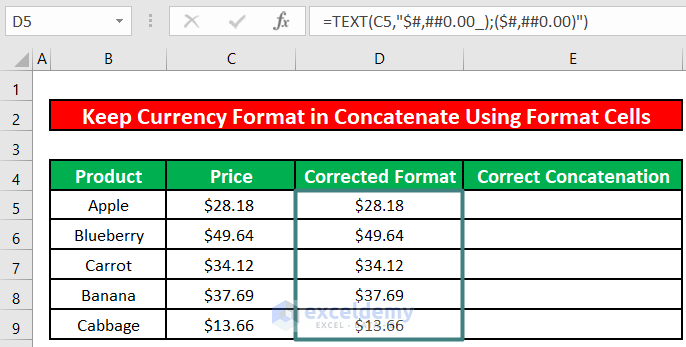
- You will see that each price value in the Price column has been formatted as currency in the Corrected Format column.
Step 4:
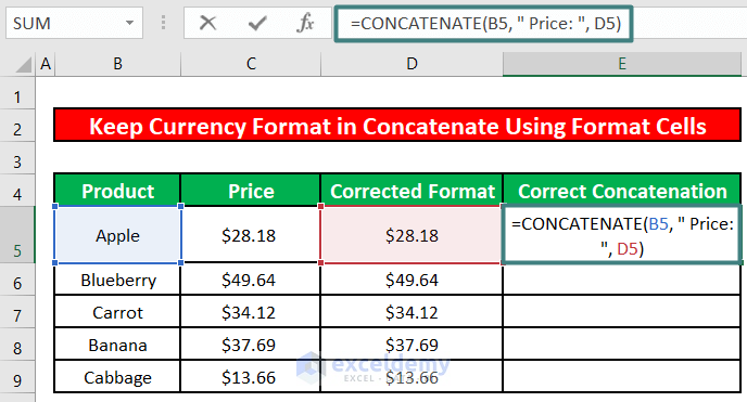
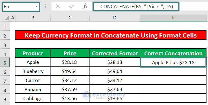
- To concatenate the product name and the corrected format of the price, enter the following formula in cell E5.
=CONCATENATE(B5, " Price: ", D5)Formula Breakdown:
The CONCATENATE function will join or concatenate the cell values B5, “ Price:“ and D5.
- Press The concatenated text will be in cell E5.
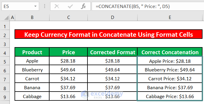
- Use the fill handle tool to apply the formula to the rest of the cells.
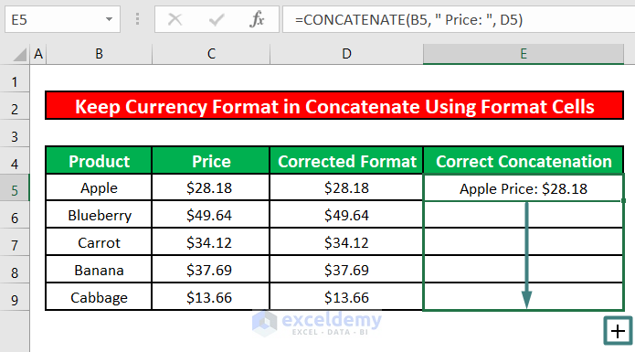
- All the concatenated text with corrected currency format will be in the Correct Concatenation column.
Method 2 – Use the Ampersand (&) Symbol to Keep Currency Format
Step 1:
- Follow the above steps to change the number format and use the TEXT function to insert the prices under the Price column in the Corrected Format column with the new number format $#,##0.00_);($#,##0.00).
Step 2:
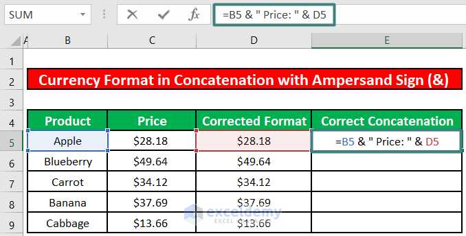
- To concatenate the product name and the corrected format of price, enter the following formula in cell E5.
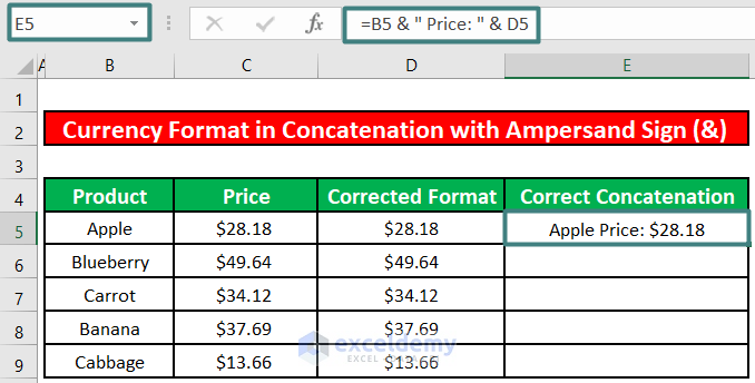
=B5 & " Price: " & D5Formula Breakdown:
The ampersand sign (&) will join or concatenate the cell values B5, “ Price:“ and D5.
- Press ENTER.
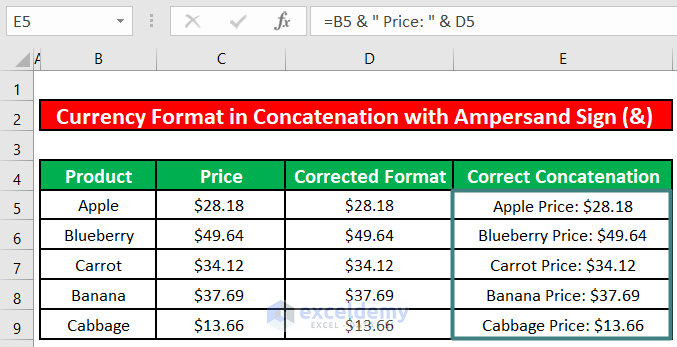
- Use the fill handle tool for the remaining cells.
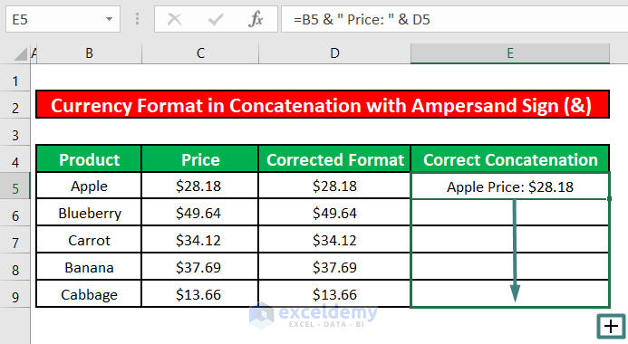
- You will see all the concatenated text with corrected currency format in the Correct Concatenation column.
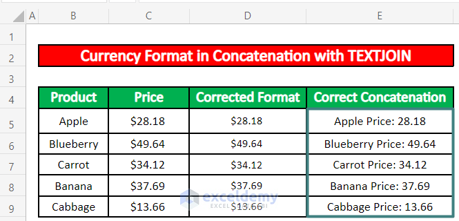
Method 3 – Perform the TEXTJOIN Function to Keep Currency Format
In Microsoft Excel 365, you can use the TEXTJOIN function to join or concatenate the text while keeping the currency format intact.
Step 1:
- Go to Format Cells and change the number format. Use the TEXT function to insert the prices in the Corrected Format column with the new number format $#,##0.00_);($#,##0.00).
Step 2:
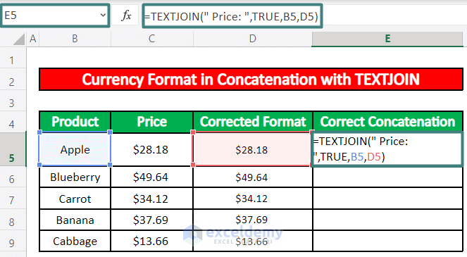
- We will concatenate the product name and the corrected format of the price. Enter the following formula in cell E5.
=TEXTJOIN(" Price: ",TRUE,B5,D5)Formula Breakdown:
The TEXTJOIN function will join or concatenate the cell values B5, “ Price:“ and D5.
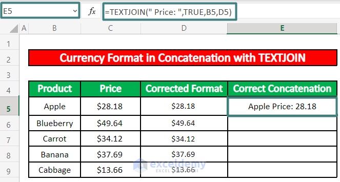
- Press ENTER.
- Use the fill handle tool for the remaining cells.
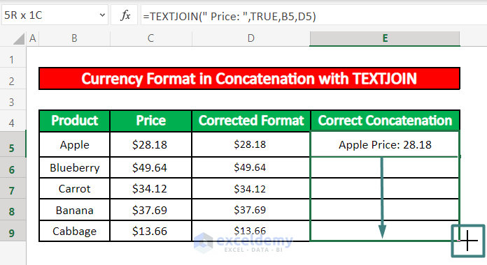
- You will see all the concatenated text with corrected currency format in the Correct Concatenation column.
Quick Notes
The CONCATENATE function is an earlier version of the CONCAT function. But both functions give the same result.
Download Practice Workbook
Related Articles
- How to Combine Text and Number in Excel
- How to Concatenate Numbers in Excel
- How to Add a 1 in Front of Numbers in Excel
- How to Concatenate Numbers with Leading Zeros in Excel
- How to Add Leading Zeros in Excel by CONCATENATE Operation
- How to Concatenate and Keep Number Format in Excel
- How to Combine Date and Text in Excel
- How to Concatenate Date That Doesn’t Become Number in Excel
- How to Combine Text and Numbers in Excel and Keep Formatting

