How to Concatenate Range in Excel (5 Useful Methods)

One of the most important features of Excel is to concatenate the values from all the cells of a range into a single cell. It is required to lookup for values with ease. Today I will be showing how to concatenate a range in Excel with 5 useful methods.

How to Concatenate Range in Excel: 5 Useful Methods

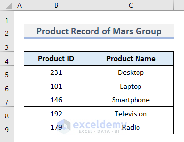
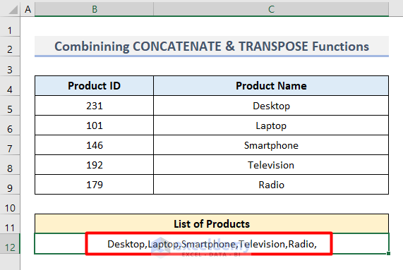
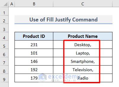
To illustrate the process, here we’ve got a dataset with the Product ID and Product Name of some products of a company named Mars Group. The values are stored in the Cell range B5:C9.

Our objective today is to concatenate the names of all the products in a single cell. For this, let’s go through the methods below.

1. Combine CONCATENATE & TRANSPOSE Functions to Concatenate Range

We can easily combine the text string by fusing the CONCATENATE and TRANSPOSE functions in Excel. To do this, follow the steps below. The CONCATENATE and TRANSPOSE functions are available in Excel 2007 or later versions.

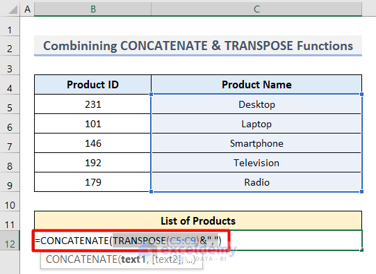
First, select Cell B12 and type this formula.

=CONCATENATE(TRANSPOSE(C5:C9&",")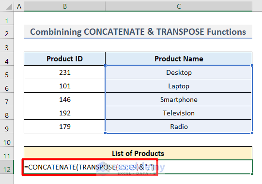

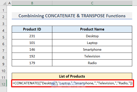
Then, select TRANSPOSE(C5:C9&”,” from the formula and press F9 on your keyboard.

Afterward, the formula will convert into values like this.
Here, remove the Curly Brackets from both sides.

In this formula, the TRANSPOSE function converts the vertical Cell range C5:C9 into a horizontal one. Following, the CONCATENATE function combines them and converts them to a single line.

Finally, press Enter and you will see the required output.

Note: Microsoft has changed how array formulas work in the version of Excel 365. In older versions, we need to press Ctrl + Shift + Enter to calculate an array formula.

2. Concatenate Range with TEXTJOIN Function in Excel

We can concatenate a range using the TEXTJOIN function of Excel. But this function is available only in Office 365. For this simply apply the steps below.

First, select Cell B12 and insert this formula.

=TEXTJOIN(",",TRUE,C5:C9)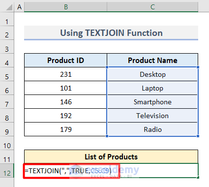

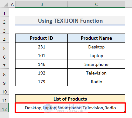
Afterward, press Enter.
Finally, you will successfully concatenate the range like this.

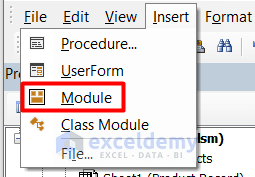
Note: Here, I set the ignore_blank argument as TRUE, to exclude the blank cells. You can use it according to your need.

3. Apply Excel VBA to Concatenate Range

Those who don’t have an Office 365 subscription, can use this VBA code to concatenate range in Excel. With this code, you can manually generate the TEXTJOIN function and concatenate it.

In the beginning, press F11 on your keyboard to open the Microsoft Visual Basic for Applications window.
Then, select Module from the Insert tab.

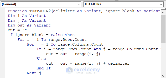
Now, type this code inside the blank page.

Function TEXTJOIN2(delimiter As Variant, ignore_blank As Variant, range As Variant)
Dim i As Variant
Dim j As Variant
Dim out As Variant
out = ""
If ignore_blank = False Then
    For i = 1 To range.Rows.Count
        For j = 1 To range.Columns.Count
            If i = range.Rows.Count And j = range.Columns.Count Then
                out = out + range(i, j)
            Else
                out = out + range(i, j) + delimiter
            End If
        Next j
    Next i
Else
    For i = 1 To range.Rows.Count
        For j = 1 To range.Columns.Count
            If range(i, j) <> "" And i = range.Rows.Count And j = range.Columns.Count Then
                out = out + range(i, j)
            ElseIf range(i, j) <> "" Then
                out = out + range(i, j) + delimiter
            End If
        Next j
    Next i
End If
TEXTJOIN2 = out
End Function

Then, press Ctrl + S to save the code and close the window.
Next, this code will generate the TEXTJOIN function with the following syntax.

=TEXTJOIN2(delimiter,ignore_blank,range)

Therefore, type the formula in Cell B12.

=TEXTJOIN2(", ",TRUE,C5:C9)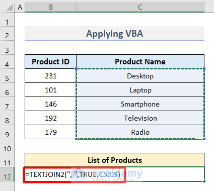

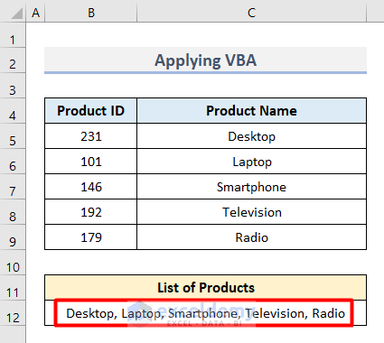
Finally, the formula will concatenate the Product Names into a single cell.

4. Concatenate Range with Power Query in Excel

Another useful method for concatenating arrays with Power Query in excel. To do the task, go through the following process carefully.

In the beginning, select Cell range C4:C9.
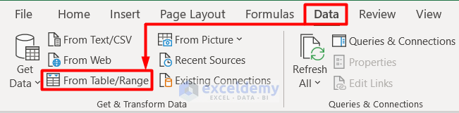
Then, go to the Data tab and select From Table/Range under the Get & Transform Data.

Following this, you will get the Create Table window asking permission to create a table with the selected range.
Here, mark check the My table has headers box and press OK.

Next, you will see the Power Query Editor window.
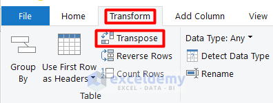
In this window, select the column and go to the Transform tab.
Here, select Transpose from the Table group.

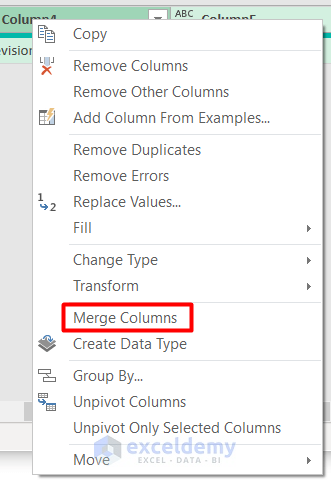
Now, select all the separated columns in the window by pressing the Ctrl button on your keyboard and right–click on any of them.
Afterward, click on Merge Columns.

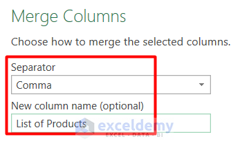
Following, choose Comma as the Separator in the Merge Columns dialogue box.
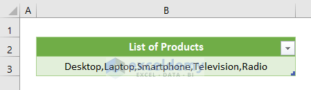
Along with it, type List of Products in the New column name section.

Lastly, select Close & Load from the Home tab.

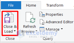
Finally, you will concatenate the range in a new worksheet like this.

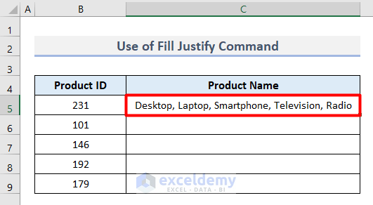
5. Use Fill Justify Command to Concatenate Range

In Microsoft Excel, Fill Justify is a rare but very useful command for concatenating. Let’s see how it works.

In the beginning, select Cell range C5:C9.

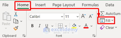
Then, go to the Home tab and click on Fill under the Editing group.

Following, select Justify from the drop-down menu.

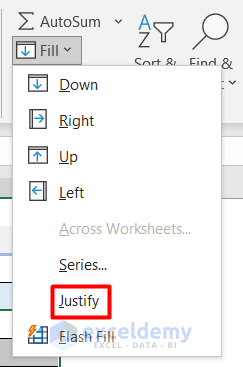
That’s it, you will successfully get the concatenated array from the single array.

Conclusion

That’s all for today. Using these 5 methods, you can learn how to concatenate a range in Excel. Do you have any questions? Feel free to ask us. Also, follow ExcelDemy for more informative articles like this.

Download Practice Workbook

Get this sample file to try the process by yourself.

Concatenate Range.xlsm

Excel Concatenate Range: Knowledge Hub

<< Go Back to Concatenate | Learn Excel

Get FREE Advanced Excel Exercises with Solutions!