Method 1 – Using the CONCATENATE or CONCAT Function to Join Multiple Columns into One Column in Excel
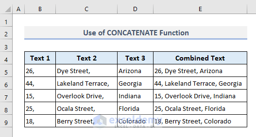
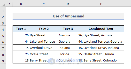
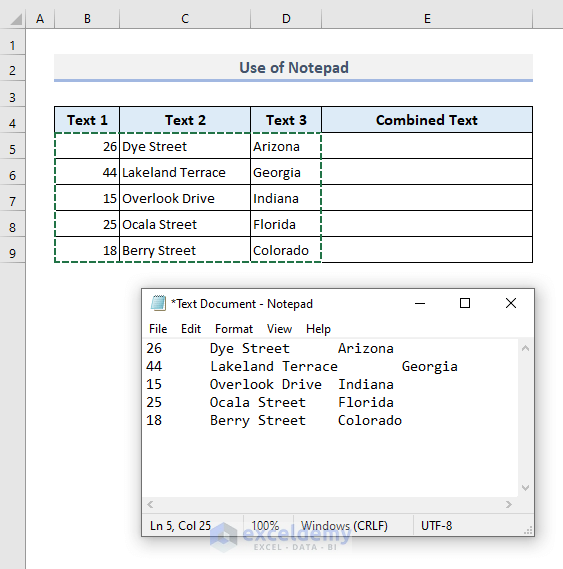
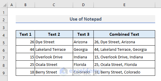
In the following picture, the three columns represent some random addresses with split parts. We have to merge each row to make an address in Column E under the Combined Text header.

- In the first output Cell E5, the required formula will be:
=CONCATENATE(B5,C5,D5)OR:
=CONCAT(B5,C5,D5)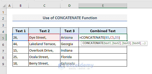
- Press Enter and drag the Fill Handle from the cell E5 down to fill the other cells.
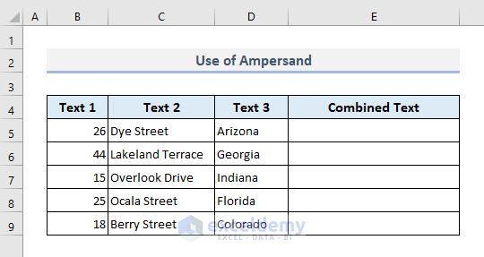
Method 2 – Inserting an Ampersand (&) to Combine Multiple Columns into a Single Column in Excel
The individual cells don’t have a delimiter, so we’ll include one.
- In the output Cell E5, the required formula is:
=B5&", "&C5&", "&D5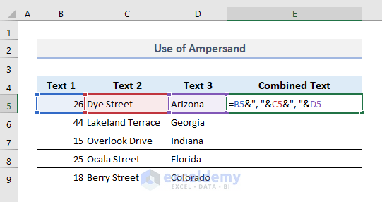
- Press Enter and autofill the entire Column E.
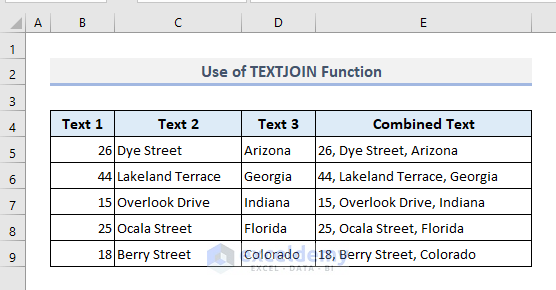
Method 3 – Inserting the TEXTJOIN Function to Combine Multiple Columns into One Column in Excel
If you’re using Excel 2019 or Excel 365 then the TEXTJOIN function is another great option to meet your purposes.
- The required formula to join multiple texts with the TEXTJOIN function in Cell E5 will be:
=TEXTJOIN(", ",TRUE,B5,C5,D5)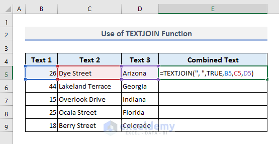
- Press Enter and drag down to the last cell in Column E.
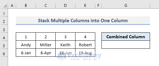
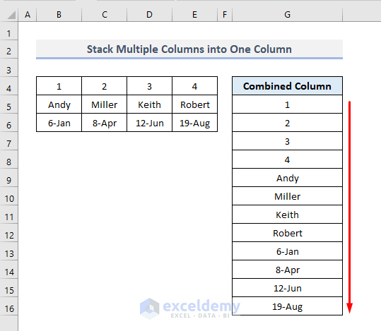
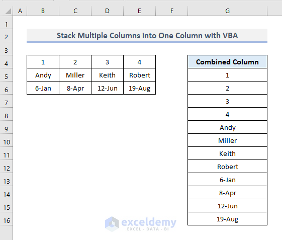
Method 4 – Stacking Multiple Columns into One Column in Excel
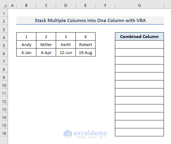
Our dataset has four random columns ranging from Column B to Column E. Under the Combine Column header, we’ll stack the values from the 4th, 5th, and 6th rows sequentially.
Steps:
- Select the range of cells (B4:E6) containing the primary data.
- Name it as Data in the Name Box (to the left of the formula bar).
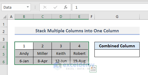
- In the output Cell G5, use the following formula:
=INDEX(Data,1+INT((ROW(A1)-1)/COLUMNS(Data)),MOD(ROW(A1)-1+COLUMNS(Data),COLUMNS(Data))+1)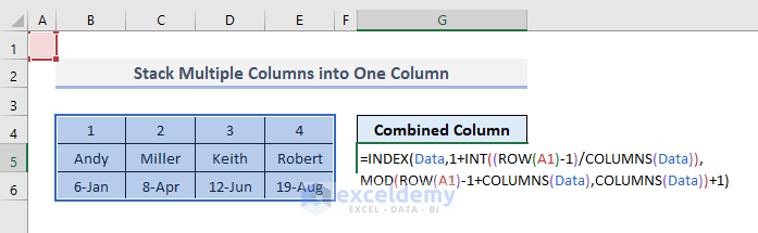
- Press Enter and you’ll get the first value from the 4th row in Cell G5.
- Use the Fill Handle to drag down along the column until you find a #REF error.
How Does the Formula Work?
- COLUMNS(Data): The COLUMNS function inside the MOD function here returns the total number of columns available in the named range (Data).
- ROW(A1)-1+COLUMNS(Data): The combination of ROW and COLUMNS functions here defines the dividend of the MOD function.
- MOD(ROW(A1)-1+COLUMNS(Data), COLUMNS(Data))+1: This part defines the column number of the INDEX function and for the output, the function returns ‘1’.
- 1+INT((ROW(A1)-1)/COLUMNS(Data)): The row number of the INDEX function is specified by this part where the INT function rounds up the resultant value to the integer form.
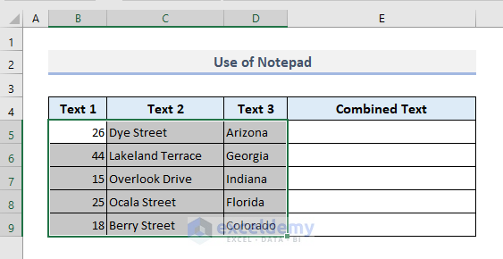
Method 5 – Using Notepad to Merge Column Data in Excel
Step:
- Select the range of cells (B5:D9) containing the primary data.
- Press Ctrl + C to copy the selected range of cells.
- Open Notepad.
- Press Ctrl + V to paste the data.
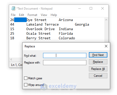
- Press Ctrl + H to open the Replace dialog box.
- Select a tab between two values in your notepad file and copy it.
- Paste it into the Find what box.
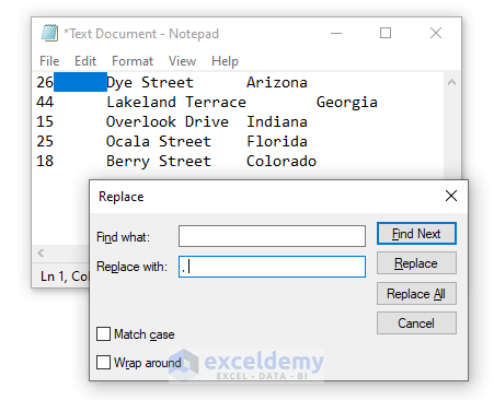
- Type “, “ (comma and space) in the Replace with box.
- Press the option Replace All.
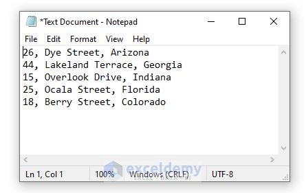
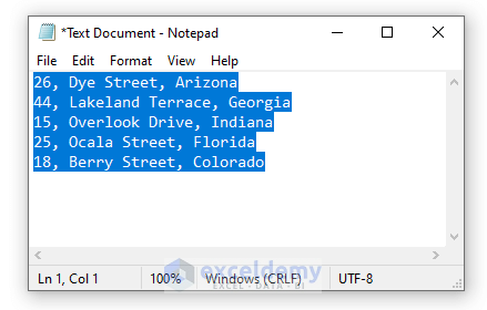
- All the data in your Notepad file will look like in the following picture.
- Copy the entire text from Notepad.
- Paste it into the output Cell E5 in your Excel spreadsheet.
Method 6 – Using VBA Script to Join Columns into One Column in Excel
In the following picture, Column G will show the stacked data.
Steps:
- Right-click on the Sheet name in your workbook and press View Code.
- A new module window will appear. Paste the following code into it:
Option Explicit
Sub StackColumns()
Dim Rng1 As Range
Dim Rng2 As Range
Dim Rng As Range
Dim RowIndex As Integer
Set Rng1 = Application.Selection
Set Rng1 = Application.InputBox("Select Range:", "Stack Data into One Column", Rng1.Address, Type:=8)
Set Rng2 = Application.InputBox("Destination Column:", "Stack Data into One Column", Type:=8)
RowIndex = 0
Application.ScreenUpdating = False
For Each Rng In Rng1.Rows
    Rng.Copy
    Rng2.Offset(RowIndex, 0).PasteSpecial Paste:=xlPasteAll, Transpose:=True
    RowIndex = RowIndex + Rng.Columns.Count
Next
Application.CutCopyMode = False
Application.ScreenUpdating = True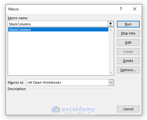
End Sub- Press F5 to run the code.
- Choose the macro name in the Macro dialog box.
- Press Run.
- Select the primary range of data (B4:E6) in the Select Range box.
- Press OK.
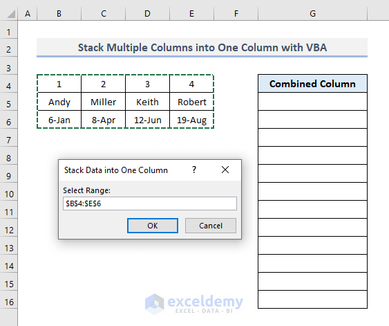
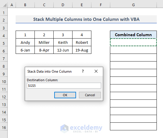
- Select the output Cell G5 after in the Destination Column box.
- Press OK.
- Here’s the result.
Download the Practice Workbook
<< Go Back to Range | Concatenate | Learn Excel
Get FREE Advanced Excel Exercises with Solutions!

Legend! Section 4 is amazing. I’ve been looking for months for this. I was using stackarray() until now but sometimes it failed. Thanks, thanks and thanks!
Hello, JUAN! Glad to know you’ve found the solutions finally from our article!
Amazing! Need little more help.
Using your formula, the result displays as
A1,B1,C1,C4,A2,B2,C2,C4….
I need the result to be displayed as per column, then next full column:
A1,A2,A3,A4,A5,B1,B2,B3,B4,B5,C1,C2,C3 and so on…
Hello, ADIL M!
Thank you for your appreciation and query.
Regarding your query, I have thought of two cases.
Case 1: Stacking all data in a single column but different rows with your desired order (A1, A2, B1, B2, and so on).
Case 2: Combining data of columns into separate cells, i.e. A1:A4 range in cell D1, B1:B4 range in cell D2, C1:C4 range in cell D3, and so on.
Download Link:
The file is attached here for you.
Solution.xlsx
⊕ 1st Case: Stacking All Data in a Single Column
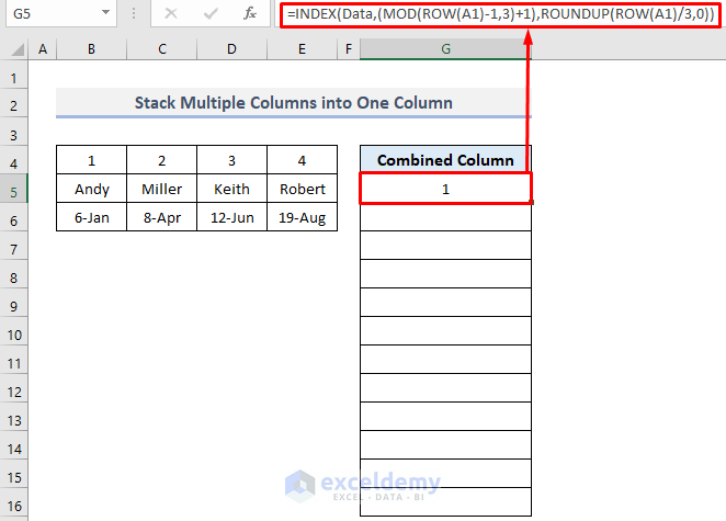
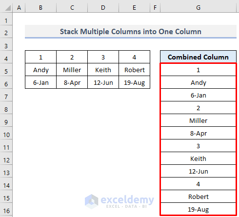
1. Use the following formula in cell G5.
=INDEX(Data,(MOD(ROW(A1)-1,3)+1),ROUNDUP(ROW(A1)/3,0))2. Following, drag the fill handle downward to accomplish your full result.
Now, this formula may look like a complex one. So, for your better understanding, I am breaking down the formula below.
Formula Breakdown:
>> MOD(ROW(A1)-1,3)
This will give you the argument of the row number in the INDEX function. If you drag the fill handle it would give you the next row numbers as per your data range.
Result: 1,2,3,1,2,3,1,2,3,1,2,3 (As our range has 3 rows and 4 columns)
>> ROUNDUP(ROW(A1)/3,0)
This part will give you the sequence of column numbers for your data range. If you drag the fill handle below you would get all the column numbers individually for all the values of your range.
Result: 1,1,1,2,2,2,3,3,3,4,4,4
>> INDEX(Data,(MOD(ROW(A1)-1,3)+1),ROUNDUP(ROW(A1)/3,0))
This will take your lookup array and generate the values individually from the lookup as per the row numbers and column numbers that you have got in the upper processes. So after dragging the fill handle below, you will get the whole data range in a single column in your desired format.
Result: 1, Andy, 6-Jan, 2, Miller, 8-Apr, 3, Keith, 12-Jun, 4, Robert, 19-Aug
⊕ 2nd Case: Combining Data of Columns into Separate Cells
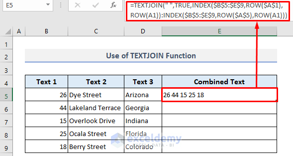
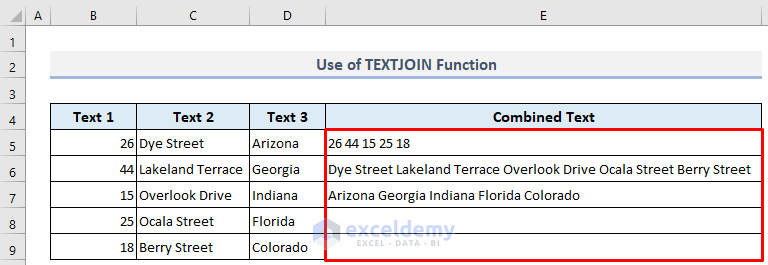
You can also use the TEXTJOIN function in this regard.
1. Insert the following formula in cell E5 now.
=TEXTJOIN(" ",TRUE,INDEX($B$5:$E$9,ROW($A$1),ROW(A1)):INDEX($B$5:$E$9,ROW($A$5),ROW(A1)))Note that the TEXTJOIN function can join an array of text. We have used the INDEX function as cell reference in the formula, to specify the array.
2. Following, drag the fill handle below to get all results.
Formula Breakdown:
>> INDEX($B$5:$E$9,ROW($A$1),ROW(A1))
This will return you the first row and first column data from your array. Here, you must reference your row_num argument with absolute reference.
Result: 26. 26 is situated in cell B5.
>> INDEX($B$5:$E$9,ROW($A$5),ROW(A1))
This will return you the last row of the following column data of your array.
Result: 18. 18 is situated in cell B9.
>> INDEX($B$5:$E$9,ROW($A$1),ROW(A1)):INDEX($B$5:$E$9,ROW($A$5),ROW(A1))
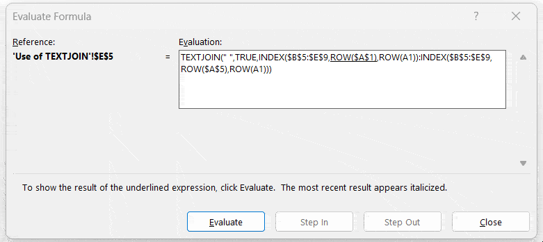
This refers to array B5:B9. To get this clearly, evaluate the formula from the Formulas tab.
>> TEXTJOIN(” “,TRUE,INDEX($B$5:$E$9,ROW($A$1),ROW(A1)):INDEX($B$5:$E$9,ROW($A$5),ROW(A1)))
This will join the texts from the first row to the last row of the first column of data with a space between each row of data.
Result: 26 44 15 25 18
Regards,
Tanjim Reza
#4 was very helpful for me. Thank you so much!
Hello Andrii,
You are welcome.
Regards
ExcelDemy