Legends are mainly used to denote the data series in an Excel chart for the convenience of our users. Sometimes, we need to show only values in the chart legends to keep it simple and good-looking. In the content, we will show you the step-by-step procedure to show legend only with values in an Excel chart. If you are interested in it, download our practice workbook and follow us.
How to Show Legend with Only Values in Excel Chart: with Easy Steps
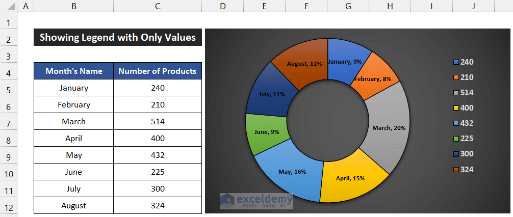
To demonstrate the procedure, we will consider a dataset of production amount per month of any industry. We are going to take the first eight months of production of any year.
Step 1: Input Required Data
In this step, we will input the number of products per month from January to August into the dataset.
- Input the name of the first 8 months in the range of cells B5:B12 and the number of products of the corresponding month in the range of cells C5:C12.

Thus, we can say that we have completed the first step to show legends with only values in an Excel chart.
Step 2: Insert Pie Chart
Now, we will insert a pie chart for our dataset. Because you can show the legends perfectly with only values in a pie chart or a doughnut chart.
- First of all, select the range of cells B5:C12.
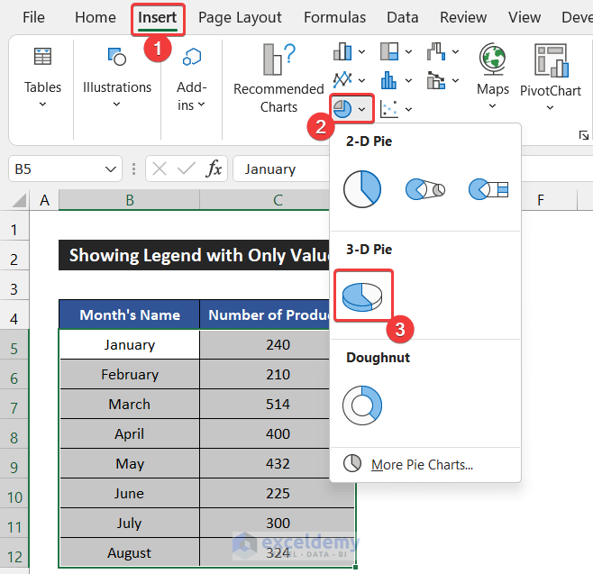
- Now, in the Insert tab, click on the drop-down arrow of the Insert Pie or Doughnut Chart from the Charts group.
- Then, choose the 3-D Pie option from the 3-D Pie section.
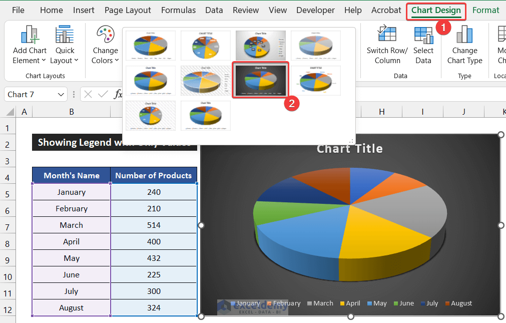
- The chart will appear on your sheet.

- You can modify your chart from the Chart Design and Format ribbons. For our chart, choose the Style 7 option from the Chart Style group.
- After that, click on the Chart Element icon and choose the chart element according to your desire.
- For our chart, we check the Data Labels and the Legends options at the right position.
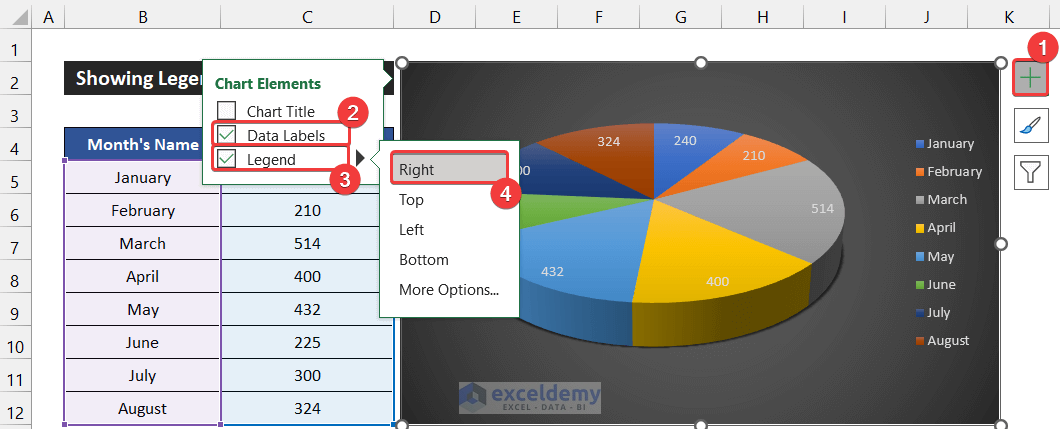
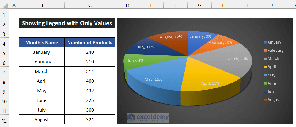
- You will see the value inside the pie chart and the month’s name in the legends. In the next step, we will show the values in the chart legends.
So, we can say that we have finished the second step to show legends with only value in an Excel chart.
Step 3: Show Legends with Only Values
In the following step, we will show the legends with only values instead of the month’s name. In addition, we are going to show the percentage and the name of the months in the Data Labels.
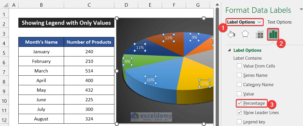
- At first, double-click on the data labels.
- As a result, a side window called Format Data Labels will appear.
- Now, in the Label Options drop-down, go to the Label Options option.
- After that, uncheck the Value option and check the Percentage option.
- You will see the data percentage in the pie chart.
- Then, to show the month’s name, check the Value From Cells option.
- As a result, a small dialog box called Select Data Label Range will appear.
- Select the range of cells B5:B12 and click OK.

- You will get the month’s name with the percentage value.
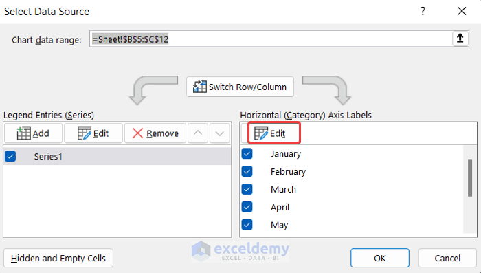
- Now, to show the value in the legends, go to the Chart Design tab and select the Select Data command from the Data group.

- A dialog box entitled Select Data Source will appear.
- Then, in the Horizontal (Category) Axis Labels, select the Edit option.
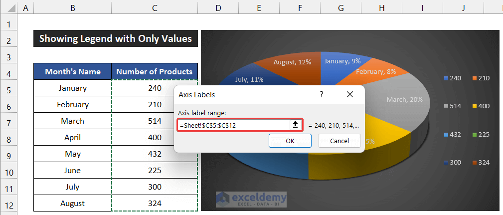
- Another dialog box titled Axis label range will appear.
- Select the range of cell C5:C12 and click OK.
- Again, click OK to close the Select Data Source dialog box.
- Modify the chart according to your desire.
- You will see the dataset value in the chart legends.
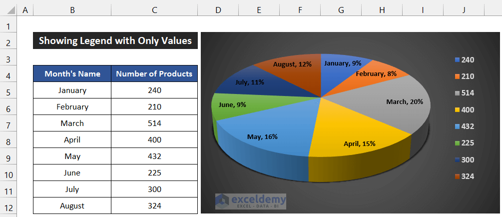
Finally, we can say that we have accomplished the final step to show legends with only value in an Excel chart.
🔍 Things You Should Know
You can also show the legends with only value in the Excel Doughnut chart. For that, in the Insert tab, choose the Doughnut chart option from the drop-down of the Insert Pie or Doughnut Chart located in the Chart group. The rest of the procedure is similar to the pie chart.
Read More: How to Ignore Blank Series in Legend of Excel Chart
Download Practice Workbook
Download this practice workbook for practice while you are reading this article.
Conclusion
That’s the end of this article. I hope that this article will be helpful for you and you will be able to show legend with only values in an Excel chart. Please share any further queries or recommendations with us in the comments section below if you have any further questions or recommendations.
Related Articles
- What Is a Chart Legend in Excel?
- How to Add a Legend in Excel
- How to Edit Legend in Excel
- How to Rename Legend in Excel
- How to Change Legend Title in Excel
- How to Change Legend Colors in Excel
- How to Reorder Legend Without Changing Chart in Excel
- How to Create a Legend in Excel without a Chart
- Excel Charts with Dynamic Title and Legend Labels
<< Go Back To Legend in Excel Chart | Excel Chart Elements | Excel Charts | Learn Excel
Get FREE Advanced Excel Exercises with Solutions!
