What Is the Legend Title in Excel?
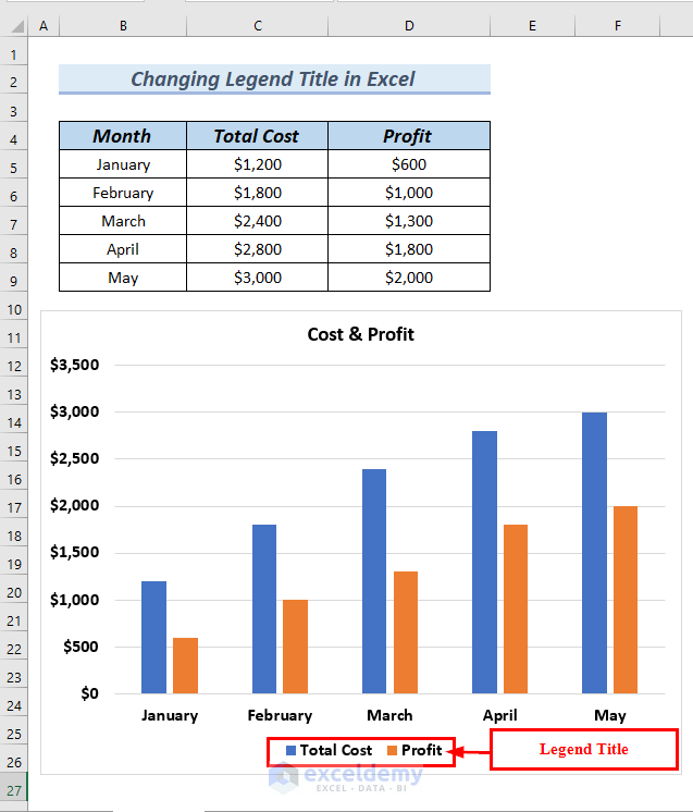
The legend title of a chart in Excel represents which data is displayed on the Y-axis (also known as Series). It usually appears on the bottom or right side of the chart. By default, legend titles are the same color as the Series values they represent. The main purpose of the legend title is to show the name and color of each data series, which prevents any confusion when readers analyze a chart or graph.
Let’s have a look at the following Column Chart based on this simple dataset. We have used the Total Cost and Profit values as Y-axis (i.e. Series) values. But it is unclear from the chart.
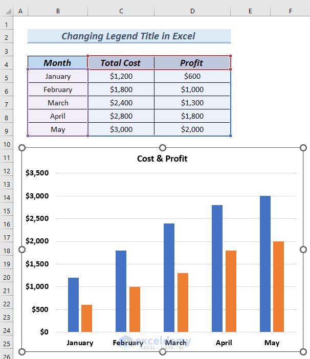
We enabled the Legend option from Chart Elements. As the legend titles are of the same color as the corresponding Series values, we can easily understand which column represents which data.
Read More: What Is a Chart Legend in Excel?
Method 1 – Editing the Main Data Table to Change the Legend Title in Excel
- To check that the legend comes from the headers of the dataset, click on the chart.
You can see that cells C4 and D4 have been used as legend titles in the chart. These are the top cells of the column of the data table.
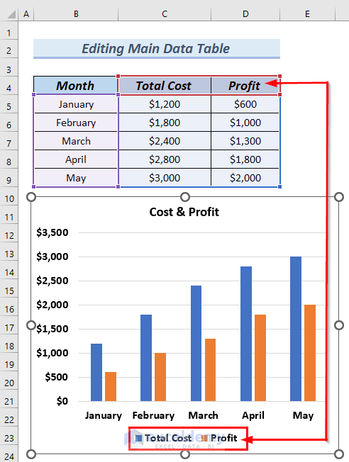
In the chart, we want to change the legend title of Total Cost to Monthly Cost. Total Cost is present in cell C4.
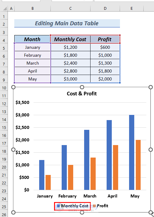
- Type a new legend title in cell C4.

- Press Enter.
You can see the legend title Monthly Cost in place of Total Cost.
Read More: How to Create a Legend in Excel Without a Chart
Method 2 – Using the Select Data Option to Change the Legend Title in Excel
You can see a column chart that has been created from the data table. The chart contains legend titles. We want to change the legend title Total Cost to Monthly Cost.

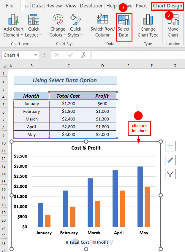
- Click on the chart.
- Go to the Chart Design tab.
- Select the Select Data option to bring out a Select Data Source dialog box.
You can also right-click on the chart and select the Select Data option to bring out the Select Data Source dialog box.
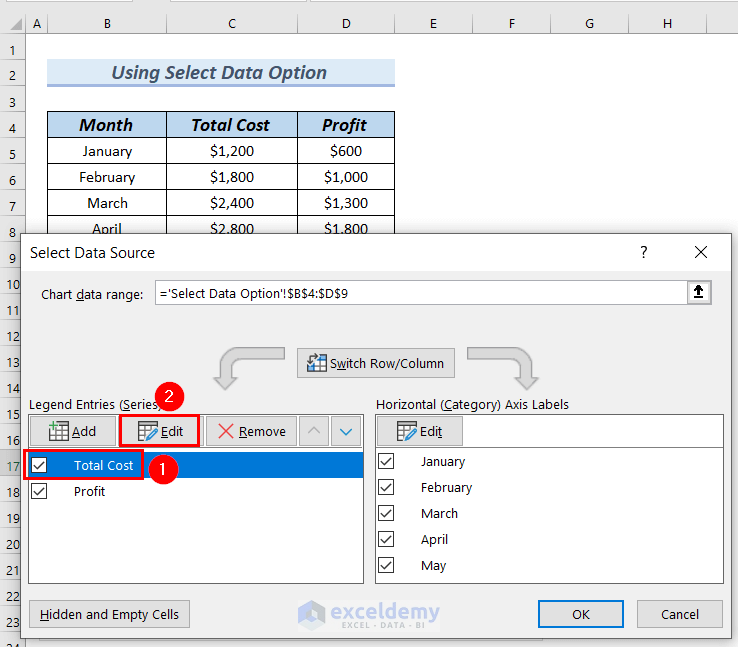
A Select Data Source dialog box will appear.
- There are two legends titled Total Cost and Profit present under the Legend Entries (Series) group.
We want to change the Total Cost legend.

- Select the Total Cost line.
- Click on the Edit option.
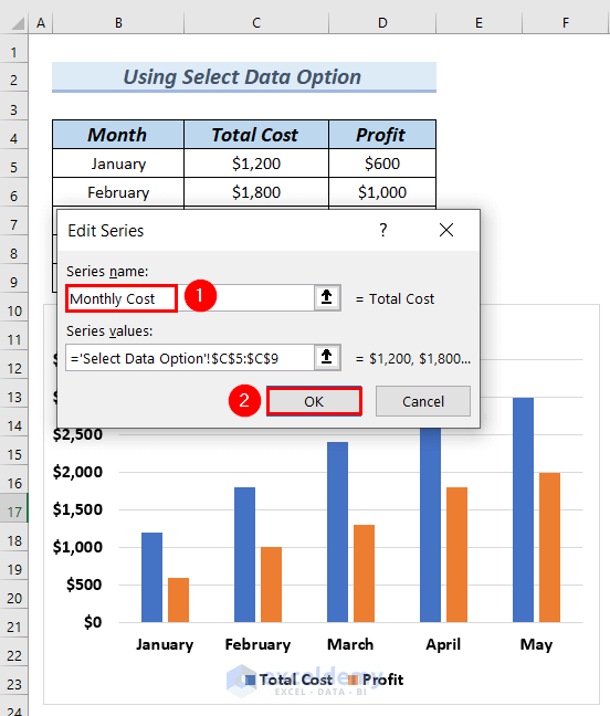
- An Edit Series dialog box will appear.
- Cell C4 is selected in the Series Name box.

- Type Monthly Cost in the Series Name box.
- Click OK.
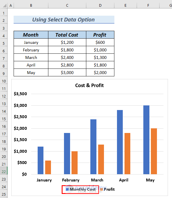
- The Select Data Source window will appear again.
Under the Legend Entries (Series), Total Cost has changed to Monthly Cost.
- Click OK.

- We get the results we needed.
Read More: How to Edit Legend in Excel
Download the Practice Workbook
Related Articles
- How to Add a Legend in Excel
- How to Change Legend Colors in Excel
- How to Reorder Legend Without Changing Chart in Excel
- How to Show Legend with Only Values in Excel Chart
- How to Rename Legend in Excel
- How to Ignore Blank Series in Legend of Excel Chart
<< Go Back To Excel Chart Elements | Excel Charts | Learn Excel
Get FREE Advanced Excel Exercises with Solutions!
