Excel is a very powerful software. We can perform numerous operations on our datasets with many different Excel tools and features. Using various charts and graphs, you can present survey results very clearly and effectively. But sometimes, blank series may be present in our dataset. And creating a chart including those blank series is not desired in most cases. Moreover, they may result in errors and can confuse the viewers. In this article, we’ll show you the step-by-step procedures to Ignore Blank Series in Legend of Excel Chart.
How to Ignore Blank Series in Legend of Excel Chart: with Easy Steps
There are many different charts and graphs in Excel that we can choose from to apply to our datasets. It depends on the user’s requirements. In this article, we’ll insert the 2-D Clustered Column Chart. This chart is useful when comparing certain outputs. Therefore, follow the steps below carefully to accomplish the job.
STEP 1: Input Data
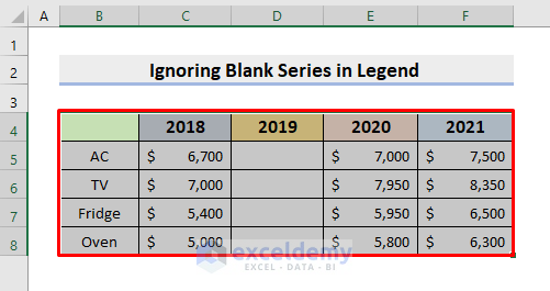
- In this example, we’ll input the name of the products and year-wise sales.
![]()
- Now, delete the sales series for the year 2019.
- Next, delete the Name header cell.
- This will avoid any complications while plotting the chart.
![]()
STEP 2: Insert Excel Chart
We will show how to insert a chart in Excel in this step. So, learn the following process to carry out the operation.
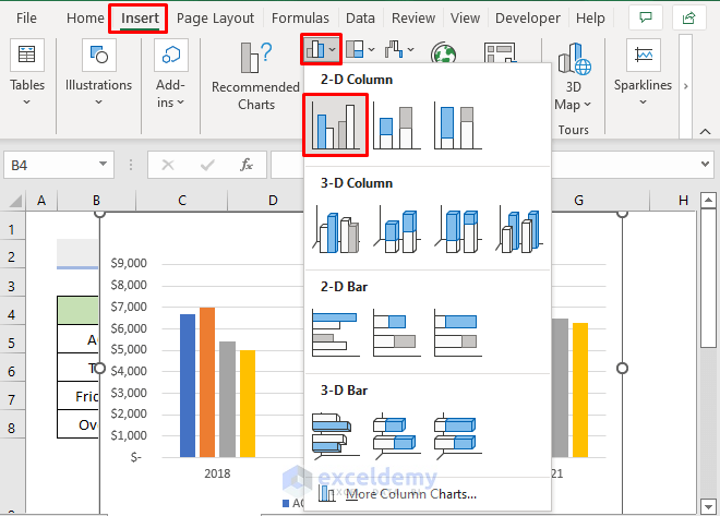
- Firstly, select the range B4:F8.
- Then, go to the Insert tab.
- After that, click the Chart drop-down icon as marked below.
- Subsequently, choose the 2-D Clustered Column chart.
- Now, click the chart.
- Consequently, in the Chart Design tab, select Switch Row/Column.
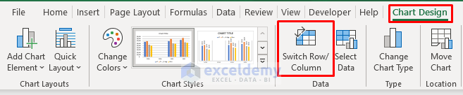
- As a result, you’ll get a 2-D clustered column chart.
- Here, the products are the Y-axis labels.
- And Years are the Legends.
- Look at the below figure to understand better.
STEP 3: Format Chart
However, you can modify and edit the chart to your requirements. In this step, you’ll know how to format the chart.
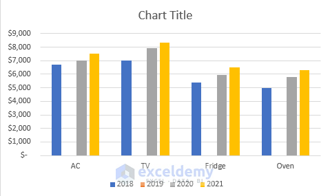
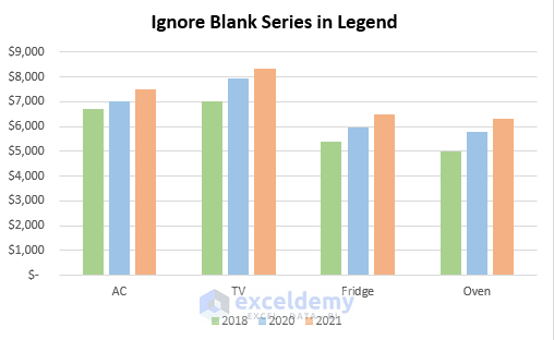
- First of all, click the Chart Title and edit the name.
- Next, select each of the series in the chart and fill it with your desired colors.
- Hence, it’ll look like the one demonstrated below.
![]()
STEP 4: Ignore Blank Series in Legend
Our main target is in this step. We’ll ignore the blank series in the legend. Therefore, follow the process.
- In the beginning, select the legend with a single click on it.
- Then, click the desired year.
- Here, we click 2019.
- Afterward, double-click on the mouse.
- As a result, the Context Menu will pop out.
- Choose Delete Series.
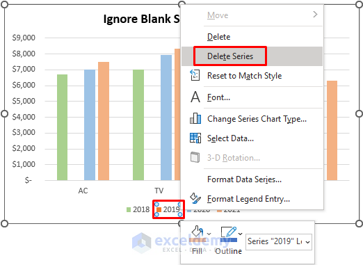
- Thus, it’ll return the chart deleting 2019 from the legend and the chart plotting too.
- So, you won’t see any gaps in the product columns.
- But, if you just want to delete 2019 from the legend only, choose the Delete option in the context menu.
- Consequently, you’ll get the chart as displayed below.
![]()
Final Output
Our chart is finally ready to present. We’ll make the last modification to make it appear more eye-catching.
- At last, we will remove the Gridlines.
- Select the Gridline and press Delete.
- Hence, the following chart gives us a comparative study of the sales of each product throughout the years.
![]()
Download Practice Workbook
Download the following workbook to practice by yourself.
Conclusion
Henceforth, you will be able to ignore blank series in the Legend of Excel Chart following the above-described examples. Keep using them and let us know if you have more ways to do the task. Don’t forget to drop comments, suggestions, or queries if you have any in the comment section below.
Related Articles
- What Is a Chart Legend in Excel?
- How to Add a Legend in Excel
- How to Edit Legend in Excel
- How to Change Legend Colors in Excel
- How to Show Legend with Only Values in Excel Chart
- How to Reorder Legend Without Changing Chart in Excel
- Excel Charts with Dynamic Title and Legend Labels
- How to Create a Legend in Excel Without a Chart
- How to Rename Legend in Excel
- How to Change Legend Title in Excel
<< Go Back To Legend in Excel Chart | Excel Chart Elements | Excel Charts | Learn Excel
Get FREE Advanced Excel Exercises with Solutions!
