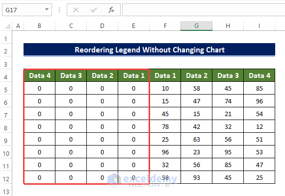
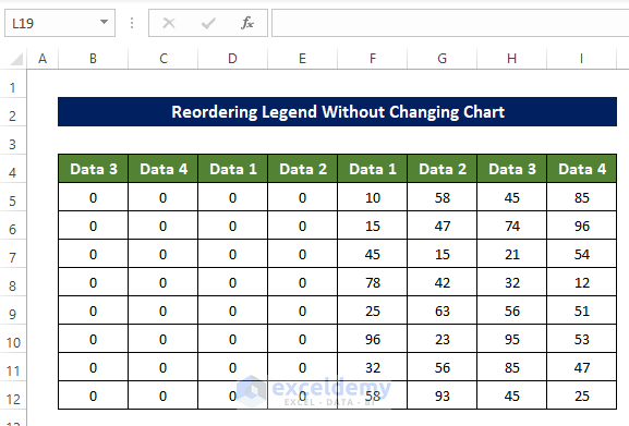
Step 1 – Add Dummy Values to Dataset
- Add dummy values to your dataset.
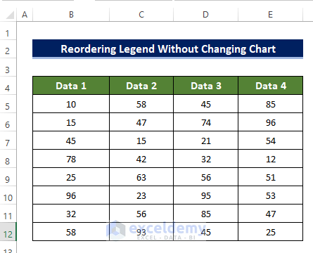
- Suppose you have a dataset with a chart whose legend you want to reorder without altering the chart itself.
- These dummy value entries should be set to zero, and the column headers must be in reverse order.
- Here’s an example of this procedure:
Step 2 – Create Stacked Chart
- Select the range of cells (e.g., B4:I12).
- Go to the Insert tab and click on 2D Column Stacked Chart.
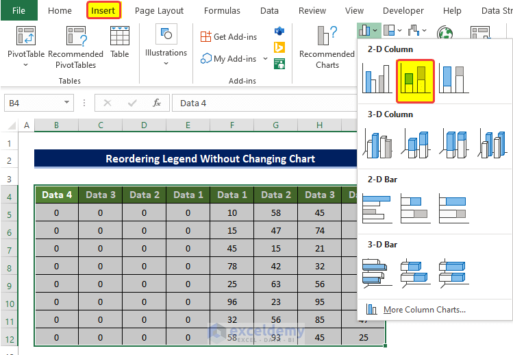
- This will create a stacked chart with the provided information.
Step 3 – Switch Row/Column
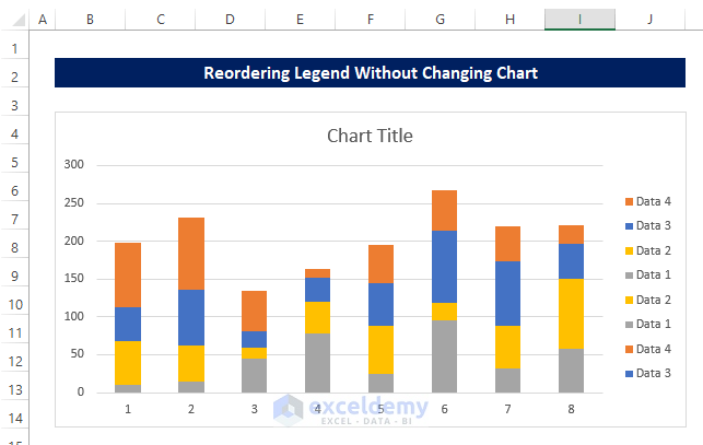
- The chart we just created may not look ideal at this point.
- To make it more usable, follow these steps:
- Select the chart and right-click on it.
- From the context menu, choose Select Data.

- In the Select Data Source window, you’ll see that the series names are listed as legend entries, and the column headers are listed as horizontal axis labels.
- Click the Switch Row/Column button.
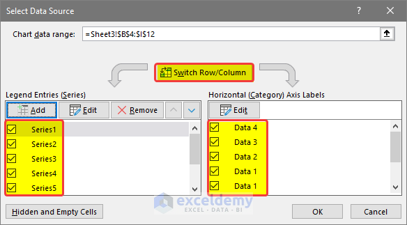
- This action will swap the legend entries with the horizontal axis labels.
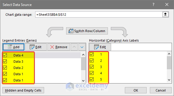
- Click OK.
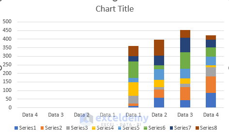
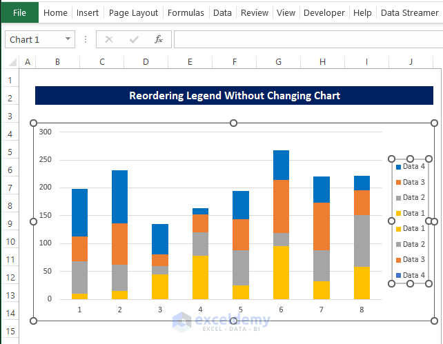
- Your chart will now resemble something like the image below:
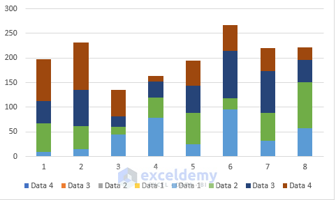
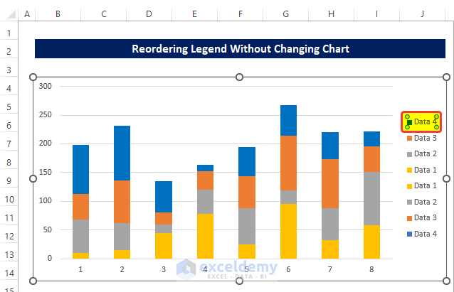
- You’ll notice that the data chart displays only 4 layers of colors, even though there are 8 different layers.
- The reason is simple: the dummy values we set to 0 have no significance in this stacked chart.
- However, all 8 data legend entries are still visible.
Step 4 – Adjust Color of Legends
Match Data Series Colors with Dummy Values:
- As we’ve prepared the chart, our next step is to ensure that the colors of the data series match those of the dummy values in the legend.
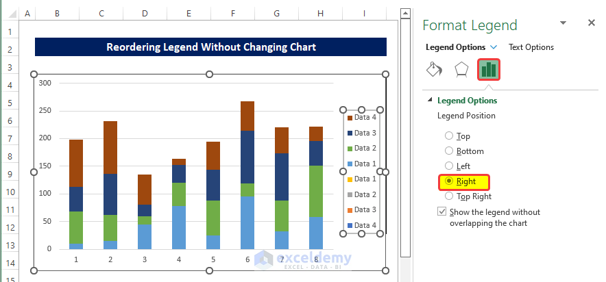
- Shift the legends to the right side of the screen:
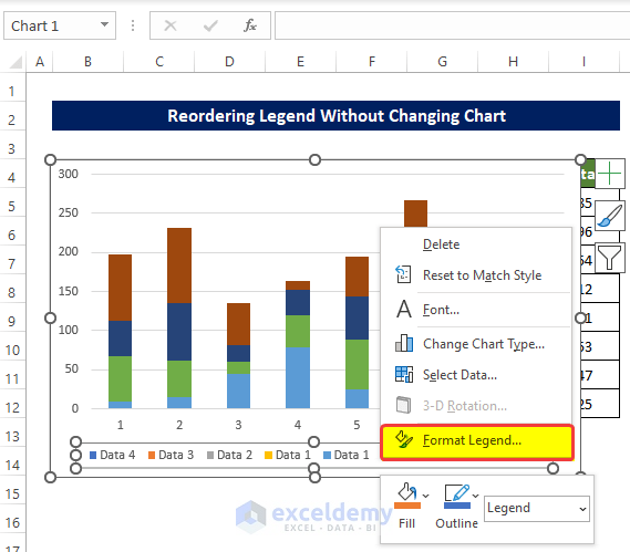
- Select the chart and right-click on it.
- From the context menu, choose Format Legend.
-
- In the Format Legends side panel options, click on Right to position the legends on the right side.
- Select the first data series (Data 4) in the chart:
- Right-click on it.
- From the context menu, click on Format Data Series.
- In the side panel, click on the color icon within the Fill & Line Options.
- Change the legend color to match Data 4 (located at the bottom of the legend).
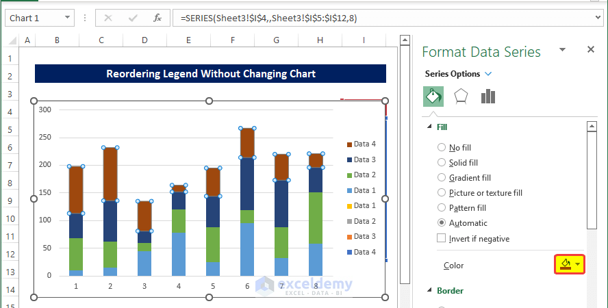
- Repeat this process for the remaining legends.
- You’ll notice that the legend entries’ colors now correspond to their respective data names.
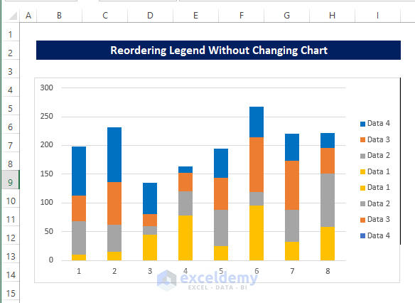
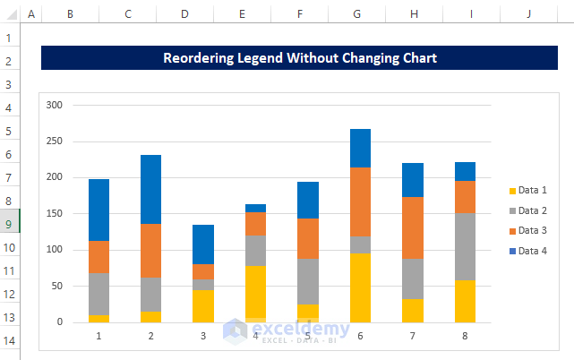
Step 5 – Remove Top Legends
- We’ve gathered all the necessary elements to reorder the legends without affecting the chart itself.
- Click on the legend area to select it.
- Double-click on the legend entry for Data 4 to select it.
- Press the Delete key to remove this entry from the chart legend.
- Repeat the same process for the other top legends in the chart.
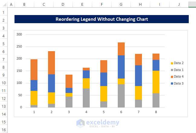
- Your chart will now resemble the image below:
- Additional Note:
- Reordering can be done in any desired order. For instance, you can reorder the legends as 2-1-4-3.
- To achieve this, set up the dummy values in the 3-4-1-2 order within your dataset.
- Follow the steps above and you’ll achieve the desired legend order.
Remember these key points
- Dummy values must be set to 0; otherwise, they may interfere with existing data.
- Arrange the desired order in the dummy value column headers. For example, if you want to reorder as 3241, arrange the column headers in the 1423 order.
Download Practice Workbook
You can download the practice workbook from here:
Related Articles
- How to Create a Legend in Excel without a Chart
- How to Edit Legend in Excel
- How to Rename Legend in Excel
- How to Ignore Blank Series in Legend of Excel Chart
- How to Add a Legend in Excel
- What Is a Chart Legend in Excel?
- How to Show Legend with Only Values in Excel Chart
- How to Change Legend Title in Excel
<< Go Back To Excel Chart Elements | Excel Charts | Learn Excel
Get FREE Advanced Excel Exercises with Solutions!
