If you are looking for how to rename legend in Excel, then you are in the right place. While using Excel, we often need to use charts of various types, where the charts are presented clearly if we use legends. Sometimes, we also need to change legend names. In this article, we’ll try to discuss how to rename legend in Excel.
What Is Legend in Excel?
In essence, legends are basically data representations. The majority of the time, when data contains uniform values across all categories, legends are used. They aid in our understanding of the data.
Read More: What Is a Chart Legend in Excel?
How to Rename Legend in Excel: 2 Ways
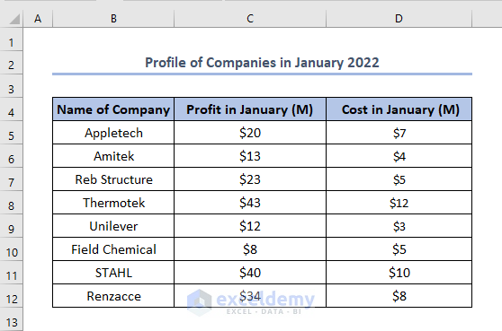
Excel offers a couple of ways to rename legends. To show this, we have made a dataset which has column headers as Name of Company, Profit in January (M), Cost in January (M). The dataset is like this.
1. Renaming Legend in Excel Dataset
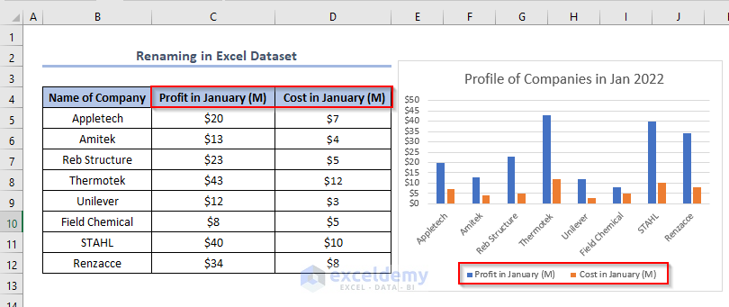
We can rename legends by working in the dataset, more specifically, in the column headers which are used as legends in the chart. Suppose, we have the following dataset and chart where Profit in January (M) and Cost in January (M) are legends. We need to rename these legends.
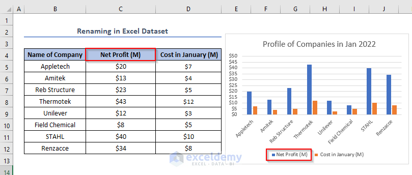
- Firstly, double-click the C4 cell and change the column header to Net Profit (M).
- Secondly, press ENTER.
- Eventually, we’ll see that the first legend of the chart is changed to Net Profit (M).
- To change the other legend, similarly, double-click the D4 cell.
- Secondly, change the column header to Net Cost (M).
- Thirdly, press ENTER.
- Consequently, we’ll see that the other legend in the chart is also changed to Net Cost (M).

Read More: How to Edit Legend in Excel
2. Using Select Data Source
We can also rename legend by using Select Data Source. When the legend needs to be distinct from the title, using Select Data Source to edit the legend is helpful. Usually, when we update the title, the legend follows suit. However, there are situations where the title can remain the same. There, this approach is appropriate.
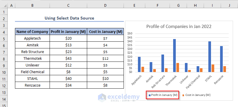
In the following figure, we need to rename the legend Profit in January (M).
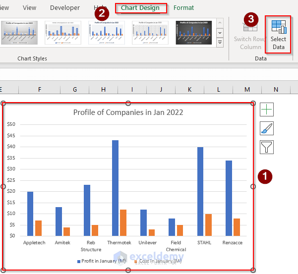
- Firstly, click on the chart.
- Secondly, go to Chart Design > choose Select Data.
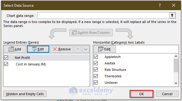
- Eventually, a Select Data Source window will appear.
- Thirdly, select Profit in January (M) > click Edit.

- An Edit Series window will appear.
- Fourthly, give a new name in the Series name box. In this case, it is Net Profit.
- Fifthly, click OK.

- Finally, again click OK in the Select Data Source window.
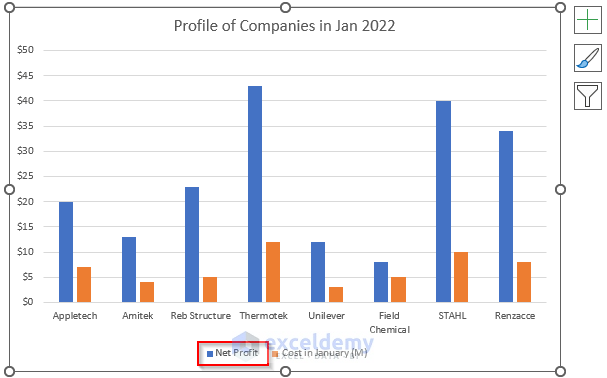
- Consequently, the first legend of the chart will change to Net Profit.
Read More: How to Create a Legend in Excel Without a Chart
How to Format Legend in Excel
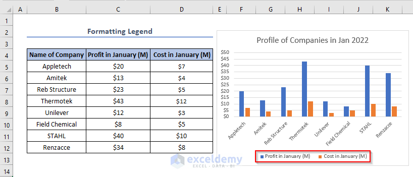
We can format legend in the chart very easily. Suppose, in the following figure, We have two legends as Profit in January (M) and Cost in January (M). We need to change the position of these legends.
- Firstly, right-click on the legend > select Format Legend.
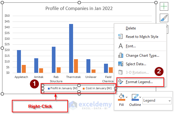
- Eventually, a Format Legend window will appear.
- Secondly, in the Legend Position box choose any of the options according to your requirements. In this case, it is Top.

- Consequently, we’ll see that the position of the legend is now on the top of the chart.

Read More: How to Change Legend Colors in Excel
How to Change Legend Name in Excel Pivot Chart
If we use the Pivot Chart in Excel, we can also change the legend of that Pivot Chart easily.
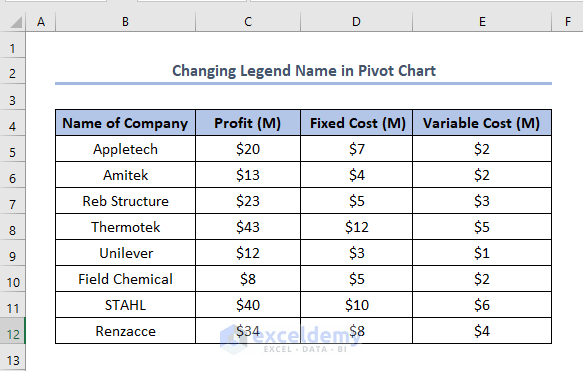
Suppose, we have the following dataset. Where Name of Company, Profit (M), Fixed Cost (M) and Variable Cost (M) are column headers. Let’s follow the instructions below to change the legend title or name!
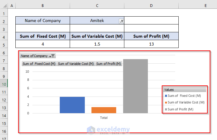
We have made a Pivot Chart based on this dataset like this. Here, the legend is Value.
We need to change the legend here. Basically, we’ll try to add another legend here to make a change.
- Firstly, click on the chart.
- Secondly, go to PivotChart Analyze > choose Field List.

- Eventually, a PivotChart Fields window will appear where we can see Values in the Legend box.

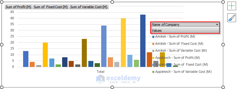
We want to add the Name of Company as a legend.
- To do this, drag the Name of Company from the Filters box and place it in the Legend (Series) box.

- Consequently, Name of Company will be added to the chart as a legend and thus the change happens.
Read More: How to Reorder Legend Without Changing Chart in Excel
Things to Remember
- If we change anything in the title which is not connected with the chart, we will see legend as unchanged. Because editing legend in Excel data must require connection between the cell which we have selected and the chart.
- Editing legend by using Select Data source is handy to use when we use various types of big data base and need to change them according to different conditions and requirements.
Download Practice Workbook
Conclusion
That’s all about today’s session. And these are the ways to rename legend in Excel. We strongly believe this article would be highly beneficial for you. Don’t forget to share your thoughts and queries in the comments section.
Related Articles
- How to Add a Legend in Excel
- How to Show Legend with Only Values in Excel Chart
- Excel Charts with Dynamic Title and Legend Labels
- How to Ignore Blank Series in Legend of Excel Chart
<< Go Back To Legend in Excel Chart | Excel Chart Elements | Excel Charts | Learn Excel
Get FREE Advanced Excel Exercises with Solutions!
