Method 1 – Inserting Dummy Values to Create a Legend Without a Chart in Excel
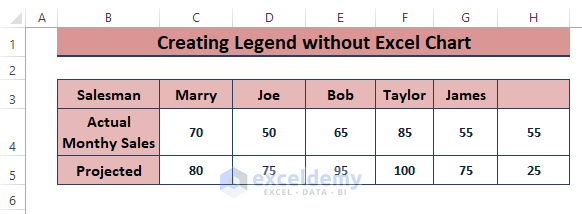
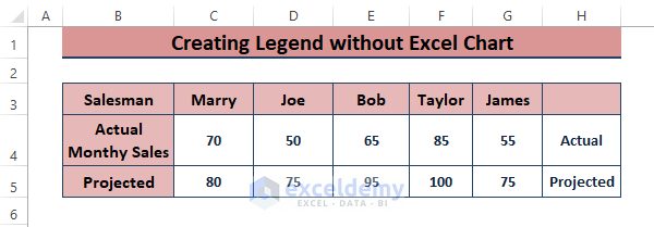
Add a helper column adjacent to the dataset. Copy the immediate cell values and paste them into the helper column cells, as shown in the image below.
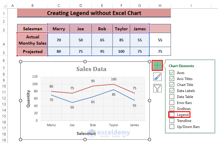
Insert a Line Chart > Display the Chart Elements (by clicking on the Plus Icon). You see, the Legend option is unticked, and the Chart displays no Legend.
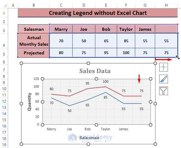
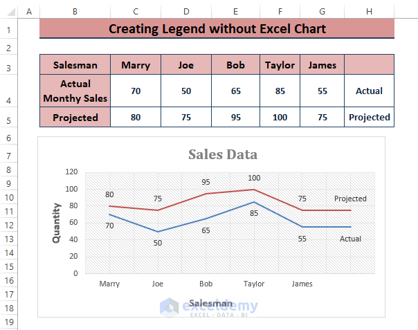
Click on the Chart, expand the Data Source range up to the dummy cells. You see, straight lines are added to the pre-existing lines, as depicted in the picture below.
Method 2 – Custom Formatting Dummy Values as Legend Names
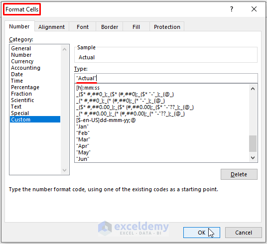
Place the cursor on the dummy value cells (here H4 and H5) and press CTRL+1 or right-click. The Format Cells or the Context Menu appears. In the case of the Context Menu, click Format Cells among the options. In the Format Cells window, select the Number section > Custom as Category > Type “Actual” (2nd time “Projected”) under Type > Click OK.
The final depiction of the dataset will be similar to the image below.
Method 3 – Inserting a Chart with Direct Legends in Excel
As the inserted Chart has expanded the Data Source (expanded in the first step), Excel automatically creates the Legend identifying the Lines without using the Chart’s option.
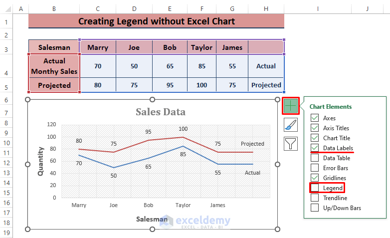
If you want to cross-check the situation, just click on the Chart > click on the Plus Icon that appears in the Side Menu > you will see the unticked Legend option. That verifies the insertion of the Legend without using a Chart in Excel. The Data Labels option is used to create a Legend within the Chart. Tick the Data Labels option from the Chart Elements.
Related Articles
- What Is a Chart Legend in Excel?
- How to Change Legend Colors in Excel
- How to Rename Legend in Excel
- How to Change Legend Title in Excel
- How to Ignore Blank Series in Legend of Excel Chart
- How to Show Legend with Only Values in Excel Chart
- How to Edit Legend in Excel
<< Go Back To Excel Chart Elements | Excel Charts | Learn Excel
Get FREE Advanced Excel Exercises with Solutions!
