How to Trim Text in Excel

Sometimes we need to trim space or character from an entire text in Excel to make the dataset attractive. We can use different Excel functions like TRIM function, RIGHT function, LEFT function, SUBSTITUTE function, REPLACE function to trim text in Excel. In this article, we are going to learn about trimming text in Excel with some examples and explanations.

Practice Workbook

Download the following workbook and exercise.

Trim Spaces from Text in Excel

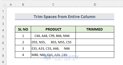
1. Trim Spaces from Entire Column Text in Excel

Assuming we have a dataset (B4:C8) of products. We are going to trim the excess spaces in between words, leading spaces & trailing spaces of all cells. The outputs will display in the D5:D8 range.

STEPS:

• First, select Cell D5.
• Now type the formula:

• Then hit Enter and use the Fill Handle tool to autofill the next cells.

2. Excel TRIM Function to Remove Space from the Left of a Text

Here we have a dataset (B5:C8) of products. We are going to use the Excel LEN function, FIND function, TRIM function & MID function to remove the left spaces from the text and return the results in the D5:D8 range.

STEPS:

• Select Cell D5 at first.
• Next type the formula:

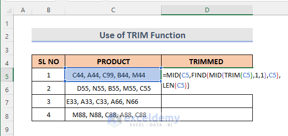
• Now press Enter and use the Fill Handle tool to see the result.

🔎 How Does the Formula Work?

• LEN(C5): This will return the string length of cell C5.
• TRIM(C5): This will trim the excess spaces in cell C5.
• MID(TRIM(C5),1,1): This will return the middle first character after trimming.
• FIND(MID(TRIM(C5),1,1),C5): This will return the position of the character we found in the previous procedure.
• MID(C5,FIND(MID(TRIM(C5),1,1),C5),LEN(C5)): This will return the extracted text without the left spaces of text.

Read more: Left Trim Function in Excel

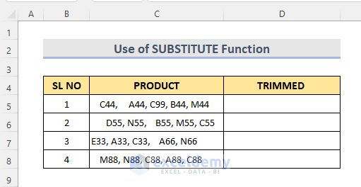
3. Trim All Space from Text in Excel with SUBSTITUTE Function

Excel SUBSTITUTE function replaces one or more characters with the given character. Let’s say we have a dataset (B5:C8) of products. SUBSTITUTE function helps us to remove all the spaces in the text string and return the result in the D5:D8 range.

STEPS:

• In the beginning, select Cell D5.
• Type the formula:

• In the end, press Enter and use the Fill Handle to the below cells.

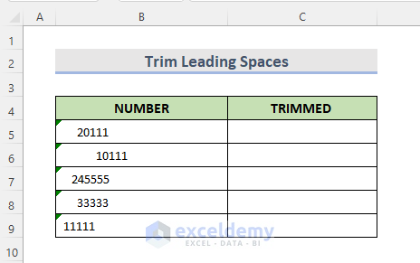
4. Trim Leading Spaces from a Numeric Column Text in Excel

To trim the spaces before the numbers in a dataset, we can use the Excel TRIM function. In dataset B4:C9, we have some numerical values.

STEPS:

• First, select Cell C5.
• Next, write down the formula:

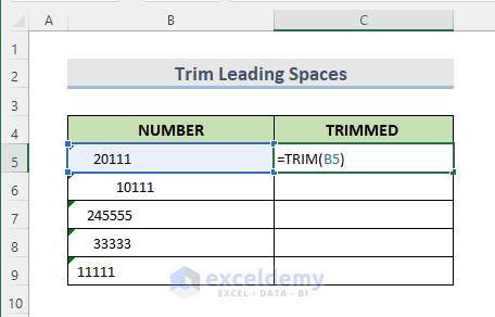
• Hit Enter and use the Fill Handle tool to see the result.

But there is a problem. All the returned values are in text values. To get the numeric value, we need to use the VALUE function with the TRIM function. The formula is:

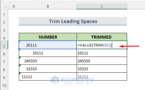
• Then press Enter and use the Fill Handle tool to apply the formula to the next cells.

5. VBA to Trim Space from Text in Excel

We can easily trim space from the dataset (B4:C8) by using Microsoft Excel VBA code. It is very easy to apply.

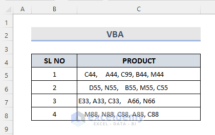
STEPS:

• Select all the values we want to trim space at first.
• Then right-click on the current spreadsheet from the sheet bar and click on the View Code option.

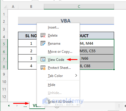
• A VBA Module window pops up.
• After that, enter the code:

Sub TRIMCELL()
Dim MyRng As Range
Set MyRng = Selection
For Each cell In MyRng
cell.Value = TRIM(cell)
Next
End Sub

• Click on the Run option now.

• Finally, we can see the result in the same column.

Trim Characters from Text in Excel

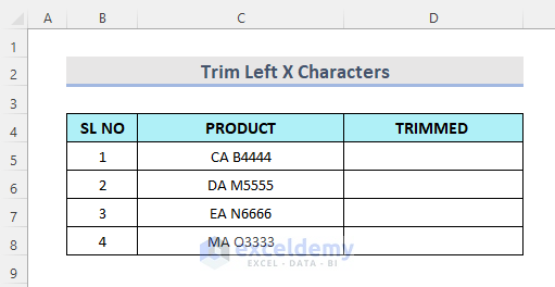
1. Trim Left X Characters from Text in Excel

Assuming we have a dataset (B4:C8) of products. We are going to use the Excel RIGHT function & LEN function to trim the left two characters from the text. The outputs will display in the D5:D8 range.

STEPS:

• First, select Cell D5.
• Now type the formula:

• Next press Enter and use the Fill Handle tool to autofill the rest of the cells.

🔎 How Does the Formula Work?

• LEN(C5)-2: This will return the number of characters after subtracting ‘2’ from the total string length of cell C5.
• RIGHT(C5,LEN(C5)-2: This will return the rightmost characters.

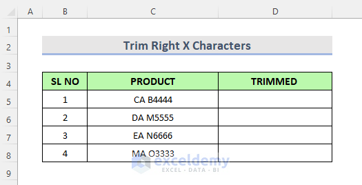
2. Right X Characters Trim from Text in Excel

Assuming we have a dataset (B4:C8) of products. We can use the Excel LEFT function & LEN function to trim the right four characters from the text and return the output in the D5:D8 range.

STEPS:

• Select Cell D5.
• Now write the formula:

• After that, hit Enter and use the Fill Handle tool to the below cells.

🔎 How Does the Formula Work?

• LEN(C5)-4: This will return the number of characters after subtracting ‘4’ from the total string length of cell C5.
• LEFT(C5,LEN(C5)-4): This will return the leftmost characters.

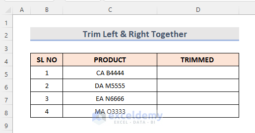
3. Trim Left & Right Characters Together from Text in Excel

Sometimes we need to trim characters from both the left & right sides of the text in excel. In this case, we need to use Excel MID function & LEN function. Here we have a dataset (B4:C8) of products.

STEPS:

• First, select Cell D5.
• Now write down the formula:

• Next hit Enter and apply the Fill Handle to the next cells.

🔎 How Does the Formula Work?

• 3+1: This will return the start position from where we want to extract the value.
• LEN(C5)-(3+4): This will return the number of characters after subtracting the total removed number (3+4) from the total string length of cell C5.
• MID(C5,3+1,LEN(C5)-(3+4)): This will return the extracted text.

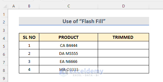
4. Use of “Flash Fill” Option

Flash Fill is an Excel built-in data tool. It is a very important feature. It automatically fills value after analyzing the previous one’s pattern. Assuming here we have a dataset (B4:C8) of products.

STEPS:

• Select Cell D5 at first.
• Now type ‘B4’ on it.
• Then start to type in the next cell. We can see that it is showing the expected values in a drop-down.

• Finally, hit Enter and we can see the whole result.

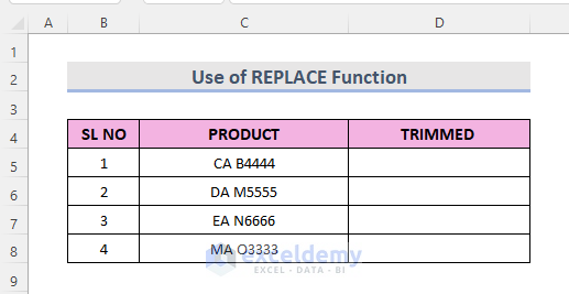
5. REPLACE Function Trimming First Characters from Text in Excel

Excel REPLACE function helps us to replace one character with the provided character. We are going to use this function to trim the first characters from text like the below dataset (B4:C8).

STEPS:

• Select Cell D5.
• Now type the formula:

• Finally, press Enter and use the Fill Handle tool to autofill the cells.

Conclusion

By using these methods, we can quickly trim text in excel. There is a practice workbook added. Go ahead and give it a try. Feel free to ask anything or suggest any new methods.

Related Readings

• Trim Right Characters and Spaces in Excel (5 Ways)