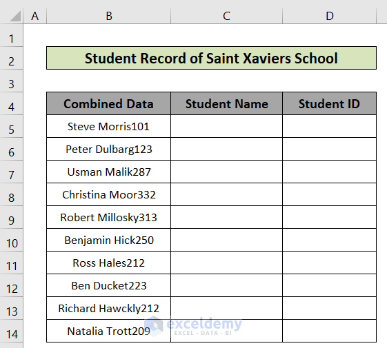
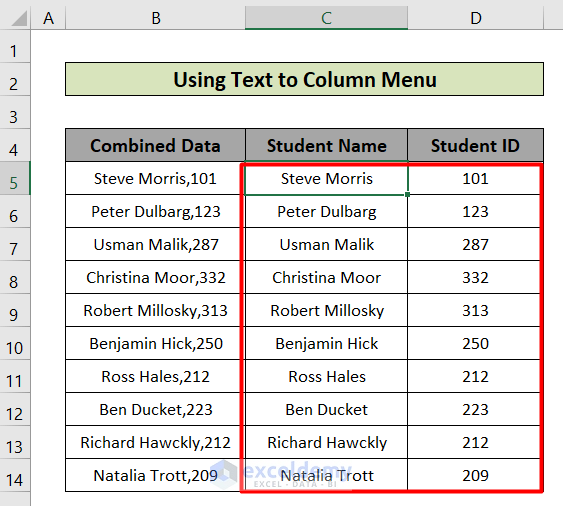
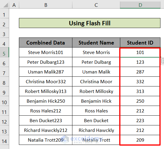
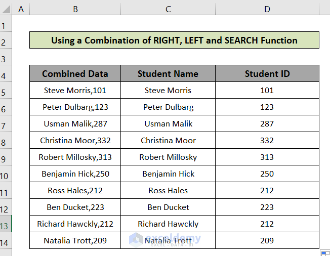
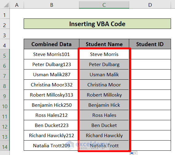
Let us have a look at this data set. We have the Combined Data of some students. We have two separate columns, C and D, where we want to extract the Student Names and Student IDs separately.
Method 1 – Using the Text to Columns Feature to Separate Text and Numbers in Excel
Steps:
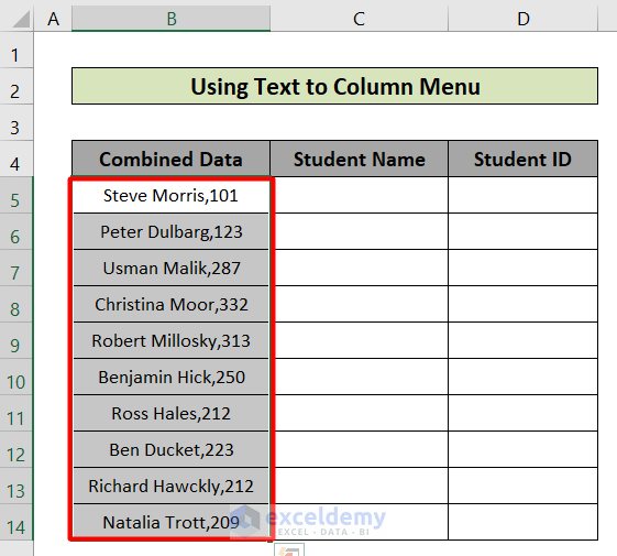
- Select the cells in which you want to separate text and numbers. We selected the range B4:B13.
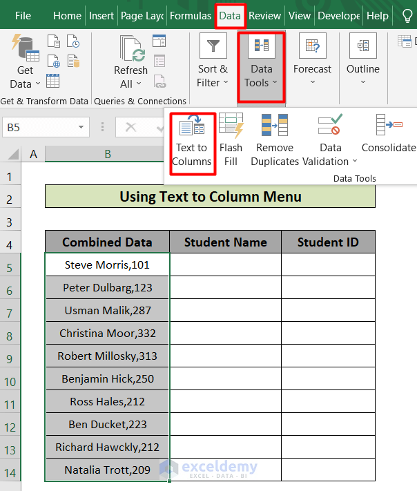
- Go to Data and choose Text to Columns under the Data Tools group.
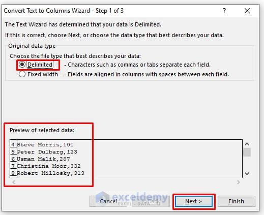
- You will get a Convert Text to Columns Wizard box. Check the Delimited option.
- You can see a preview of your data.
- Click Next.
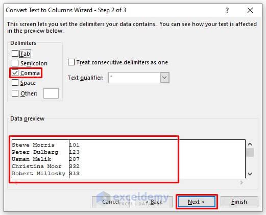
- Choose Comma from the Delimiters option. You can choose multiple Delimiters together.
- You will see a preview of your data being split.
- Click Next.
- At the bottom of the box, your data is split based on the delimiter.
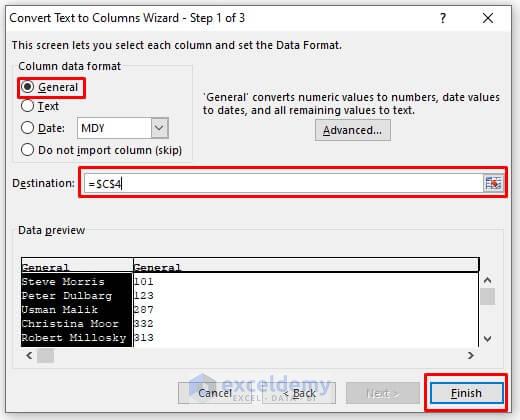
- Select each column and, in the Column data format option, select the format in which you want to have that column. We want both columns to be in General format.
- In the Destination box, put the Absolute Cell Reference of the leftmost cell of the range where you want your data to be split, or click on the small box on its right and manually select the leftmost cell of the Destination range. We selected cell $C$4.
- Click on Finish.
- You will find the Student Names and IDs split into two columns.
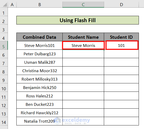
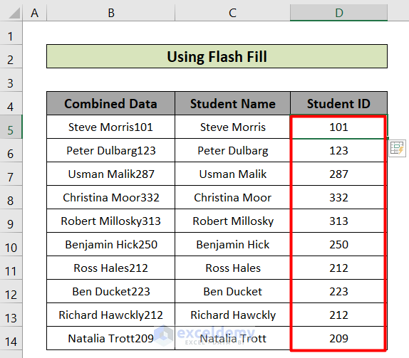
Method 2 – Separating Text and Numbers in Excel with Flash Fill
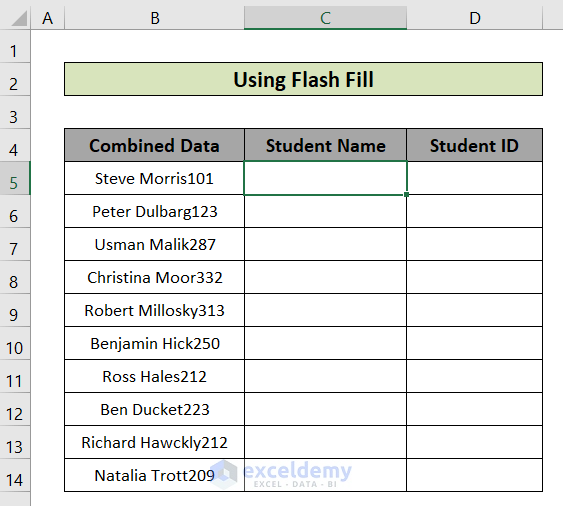
In this case, we don’t have a clear delimiter.
Steps:
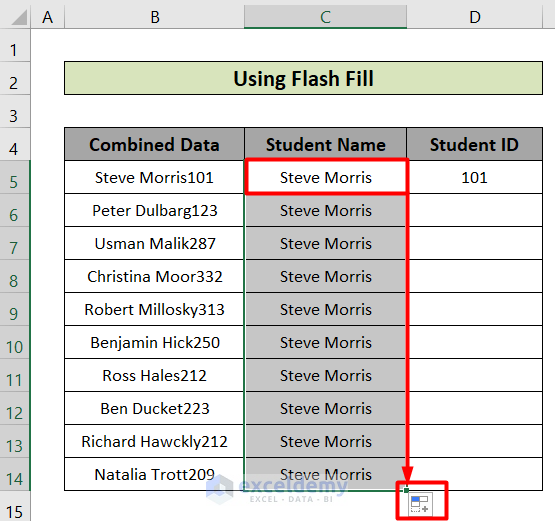
- Separate the first data point manually. We put Steve Morris in cell C4 and 101 in cell D4.
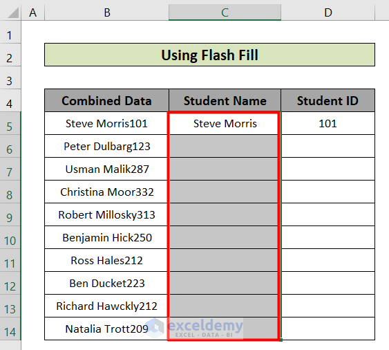
- Select the rest of the cells in the first column.
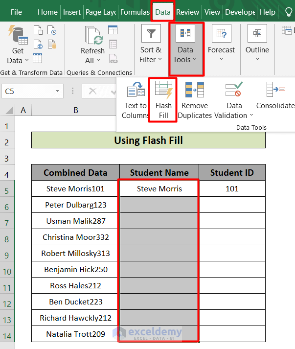
- Go to Data and select Flash Fill under the Data Tools section.
- Click on Flash Fill.
- Flash Fill will notice a pattern and fill in the values.
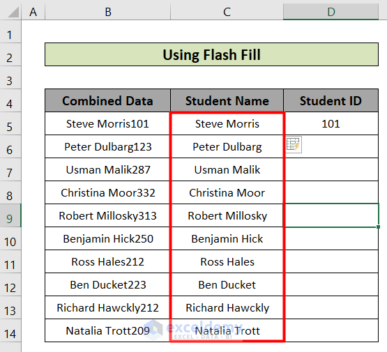
- Repeat the Flash Fill for column D.
Method 3 – Using Flash Fill via the Fill Handle to Detach Text and Numbers in Excel
Steps:
- Separate the first cell manually. We put Steve Morris in cell C4 and 101 in cell D4.
- Drag the Fill Handle of the first column through the rest of the cells. You will get a small icon called Auto Fill Options in the bottom right corner after dragging.
- Click the drop-down menu on the bottom-right.
- Click on Flash Fill.
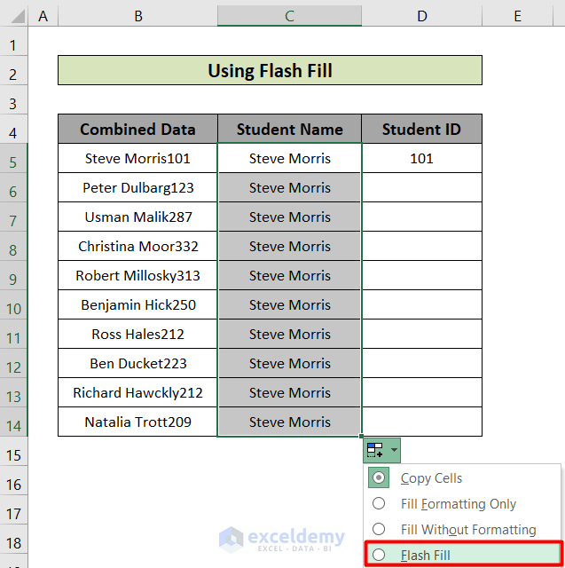
- Flash Fill will fill in the values.
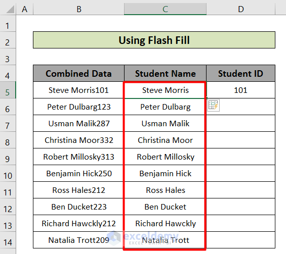
- Repeat for column D.
Note: Flash Fill is available from Excel 2013.
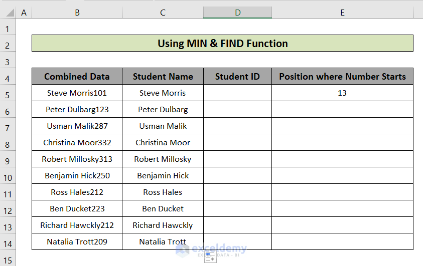
Method 4 – Detaching Text and Numbers by Inserting Excel MIN and FIND Functions
Steps:
- Use the following formula in cell E5.
=MIN(FIND({0,1,2,3,4,5,6,7,8,9},B5&"0123456789"))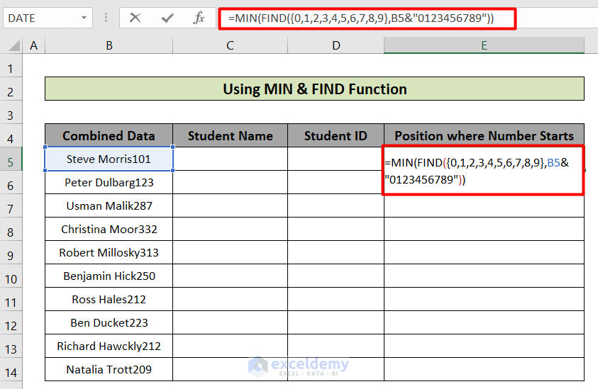
- The FIND function takes input {0,1,2,3,4,5,6,7,8,9}.
- This finds the value in cell B5 with the number starting with 0123456789.
- The MIN function returns the minimum value from the result of the FIND function.
- In the text Steve Morris101, numbers start from the 13th position.
- The formula for separating the Name will be:
=LEFT(B4,MIN(FIND({0,1,2,3,4,5,6,7,8,9},B4&"0123456789"))-1)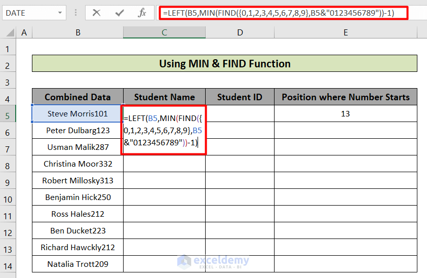
The LEFT function takes the arguments from cell B5, and the MIN, and FIND functions return the left value of B5.
- Hit Enter to apply the formula and get the name.
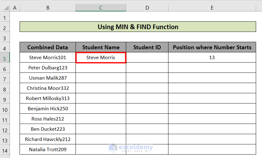
- Drag the Fill Handle to separate names for the rest of the cells.
- For the Student IDs, the formula will be:
=RIGHT(B4,LEN(B4)-MIN(FIND({0,1,2,3,4,5,6,7,8,9},B4&"0123456789"))+1)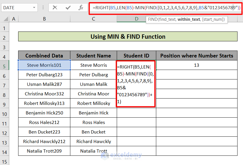
The RIGHT function takes the arguments from cell B5, and the MIN, and FIND functions return the rightmost value of B5.
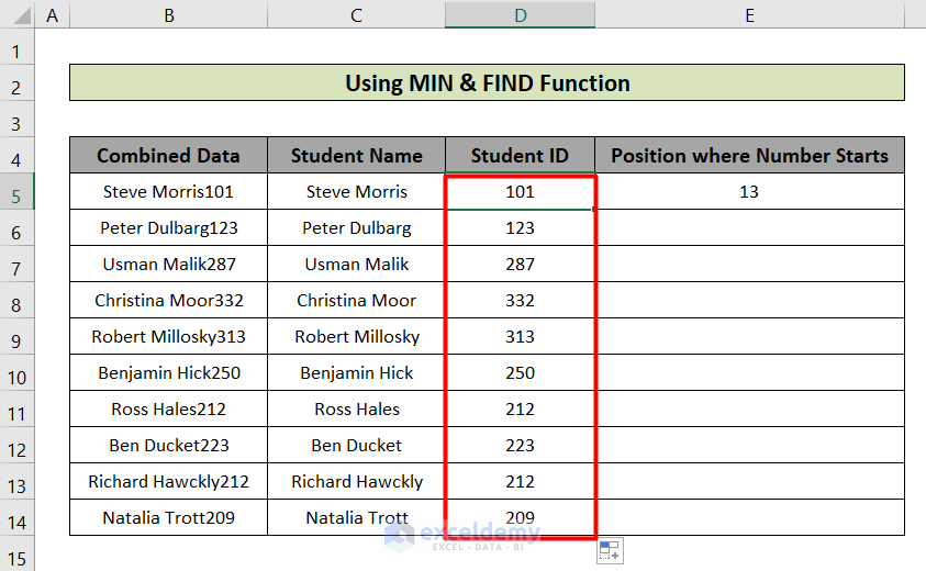
- Drag the Fill Handle. You will get the Student IDs separated as well.
- You can clear column E.
Note: If you have numbers first and text after that in the combined data, like 101Steve Morris, then the formula for the numbers will be exchanged with the formula for the text. And you have to use the MAX function in lieu of the MIN function.
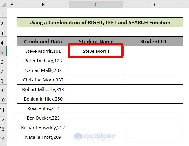
Method 5 – Combining RIGHT, LEFT, and SEARCH Functions to Separate Text and Numbers
Steps:
- Here’s the formula for separating the name for cell C5.
=LEFT(B5,SEARCH(",", B5)-1)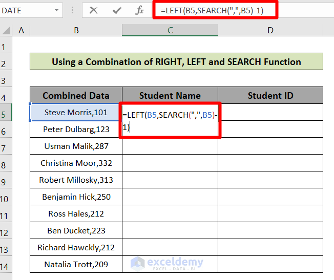
- The SEARCH function searches the comma (,) in cell B5 and returns the position number.
- The LEFT function returns the number of characters from the left side based on the value of the SEARCH function.
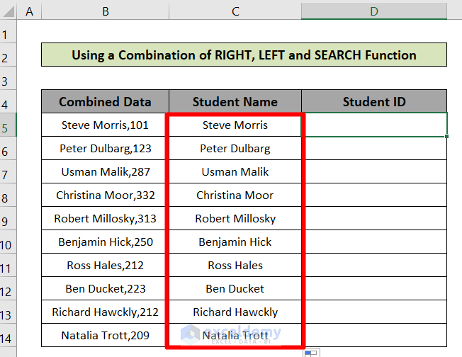
- Insert the formula and apply it with Enter.
- Use the Fill Handle to copy the formula down.
- The formula for separating the IDs in cell D5 will be:
=RIGHT(B5,LEN(B5)-SEARCH(",",B5))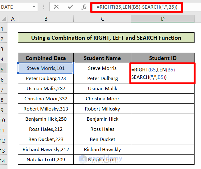
- The SEARCH function searches the comma (,) in cell B5 and returns the position number.
- Then, subtract this value from the return of the LEN function.
- The RIGHT function returns characters based on the subtraction result.
- Apply the formula.
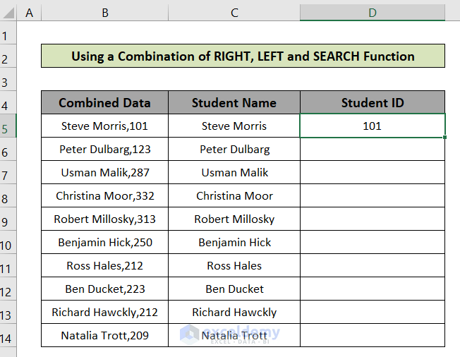
- AutoFill the column.
Note: If you have numbers first, and then text, like 101Steve Morris, then you have to exchange the formulas.
Method 6 – Applying Excel VBA Macro to Separate Text and Numbers
Steps:
- Press Alt + F11. You will get the VBA window.
- Go to the Insert tab in the VBA toolbar.
- Choose Module.
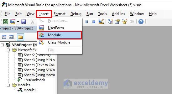
- You will get a new Module window.
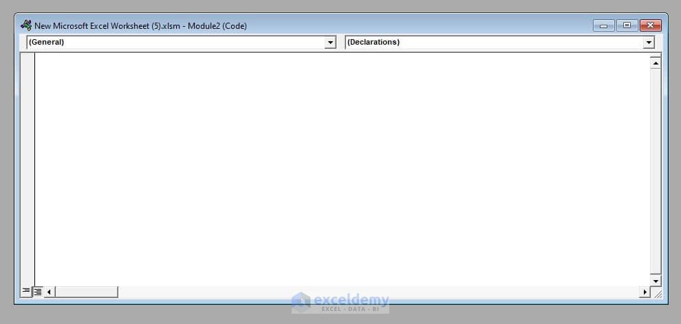
- Insert the following code here.
Public Function SplitText(pWorkRng As Range, pIsNumber As Boolean) As String
'Updateby Extendoffice
Dim xLen As Long
Dim xStr As String
xLen = VBA.Len(pWorkRng.Value)
For i = 1 To xLen
    xStr = VBA.Mid(pWorkRng.Value, i, 1)
    If ((VBA.IsNumeric(xStr) And pIsNumber) Or (Not (VBA.IsNumeric(xStr)) And Not (pIsNumber))) Then
        SplitText = SplitText + xStr
    End If
Next
End Function
Thecode creates a new function called SplitText(), which takes two arguments, a combined data and a Boolean value (TRUE or FALSE)
- Save the document as an Excel Macro Enabled Worksheet.
- Come back to your worksheet.
- In cell C4, insert this formula:
=SplitText(B4,FALSE)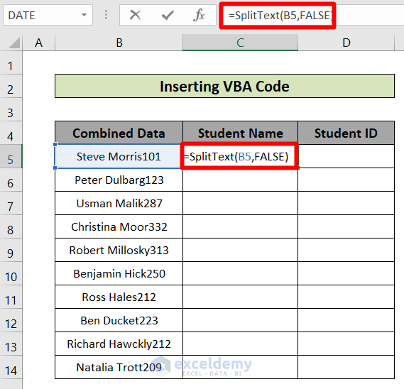
- You will get the names separated.
- In the Student ID column, insert this formula.
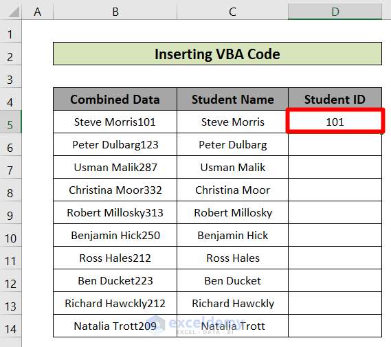
=SplitText(B4,TRUE)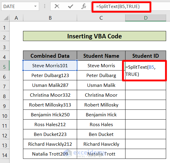
- You will get the Student IDs separated.
- AutoFill the columns.

Special Note: The VBA can separate numbers and text from data where everything is mixed randomly. For example, it can separate 101 and Steve Morris from Steve10 M1orris, which the other methods can’t.
Download the Practice Workbook
Separate Text and Numbers: Knowledge Hub
<< Go Back to Split | Learn Excel
Get FREE Advanced Excel Exercises with Solutions!

Really Usefull, Thank you
hi, is there any method to separate a mix of numbers and letters automatically? like in chemical equations Cr11C8H18: Cr=11, C=8 and H=18
Greetings 3ADDOULA MA5ASSAK, thank you for your question. I hope the following codes will solve your issue.
However, if this doesn’t solve your problem, you can mail us your Excel file with detailed instructions to: [email protected], and we’ll try to solve it as soon as possible.
28 February 2025
Thanks for this article.
I just found the TEXTAFTER and TEXTBEFORE functions. These are good because you can use a negative value of the sought character instance number to start searching from the right hand end of a string. Powerful and useful when you have unstructured strings with a mix of text, numbers and spaces.
Hello Chris,
You’re absolutely right! TEXTAFTER and TEXTBEFORE are powerful functions, especially for handling unstructured text. The ability to use a negative instance number for searching from the right makes them even more versatile. Thanks for sharing this insight!
Thanks for sharing your valuable insight.
Regards
ExcelDemy