[Fixed!] NAME Error in Excel (7 Reasons with Solutions)

Excel is a powerful tool widely used for data analysis, organization, and reporting. While working with formulas and functions, you may come across a common hurdle known as name error in Excel.
Understanding the causes of name error, their implications, and how to resolve them is crucial for ensuring accurate calculations and maximizing efficiency.
In this guide, we will explore the world of name error in Excel and provide easy-to-implement solutions to overcome them effectively. Let’s dive into name error in Excel together.

What Is #NAME Error in Excel

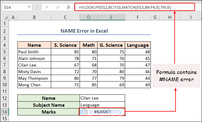
The #NAME error occurs in Microsoft Excel when a formula includes a function or range name that is unrecognized or misspelled. Excel cannot interpret a text string within the formula as a valid component, resulting in this name error message.
If, for instance, you mistakenly provide an incorrect cell reference, Excel will be unable to recognize it and will generate a #NAME error. The cell containing the formula will display the error message, hindering the formula from producing a valid outcome.

[Fixed!] NAME Error in Excel: 7 Valid Reasons with Solutions

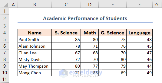
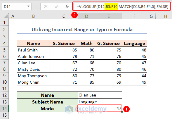
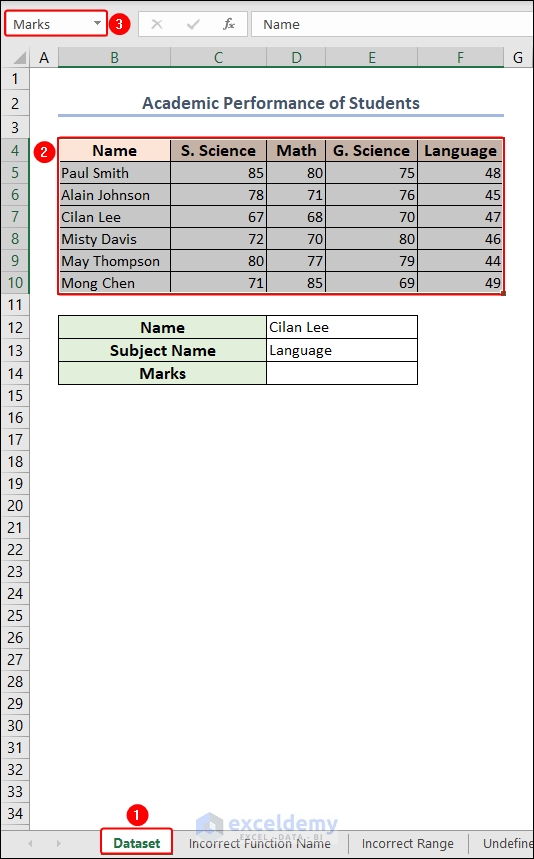
Let’s assume we have a sheet of the Academic Performance of Students of a specific institution. This dataset includes Name and their marks for different subjects like S. Science, Math, G. Science, and Language under columns B, C, D, E, and F respectively.

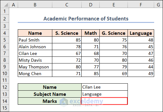
Here, we will find out the marks of a certain subject of a specific student in cell D14 by using a formula in Excel. To do this, we’ll use the VLOOKUP and the MATCH functions.

Now, we’ll utilize this dataset to show reasons for #NAME errors in Excel using multiple examples. We’ll show the corresponding solutions to them too. So, let’s explore them one by one.
Not to mention, here, we have used the Microsoft Excel 365 version; you may use any other version according to your convenience. Please leave a comment if any part of this article does not work in your version.

Reason 1: Using Incorrect Function Name Will Cause #NAME Error

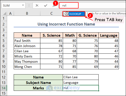
Let’s say, you want to get the Marks for Cilan Lee in Language using the VLOOKUP function. But you got here the #NAME error due to typing a wrong function name like this example. Here, we typed it as VLOOKOP instead of VLOOKUP.

The formula we put in cell D14 is the following:

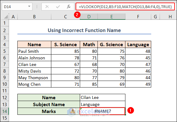
Solution: Utilize Formula AutoComplete Feature

To get rid of the error, you can use Formula AutoComplete to have the right function name and structure in the formula.

• At first, write the initial one or two letters of the function name in the Formula Bar and Excel will suggest various functions. From the list, select your preferred function and press the TAB key to bring the function into operation.

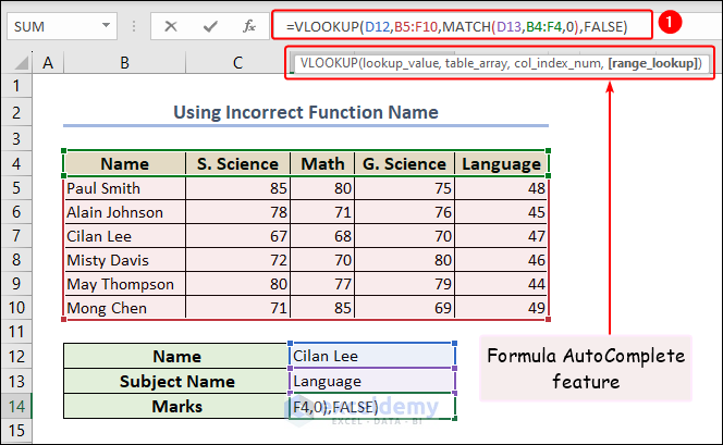
• Now, you can see the arguments of the function while giving inputs into the formula. It’ll help to give correct inputs. After completing the formula, press the ENTER key.

Behold, Excel eliminated the NAME error, and the cell (D14) now displays the correct output.

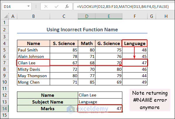
In this process, you don’t have to write the full function name. As a result, the percentage of errors gets reduced.

Reason 2: Utilizing Incorrect Range or Typo in Formula

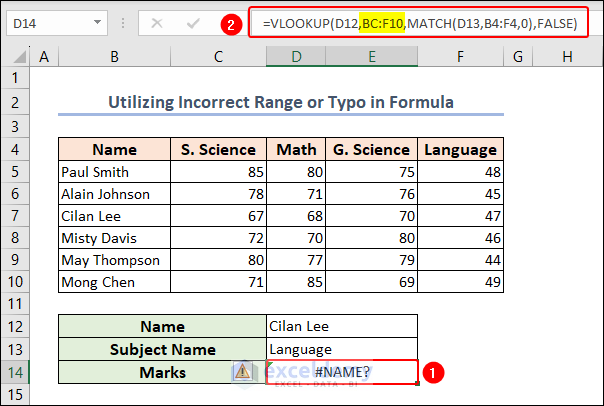
Here, we want to get output like Example 1. But, it’s showing the #NAME error in the output cell (D14). We employed the following formula to accomplish the task.

Look, we gave BC:F10 in the table_array argument of the VLOOKUP function. That’s the reason behind showing errors in Excel.

Solution 1: Select Range Instead of Typing in Formula

While typing the range in a formula you may sometimes miss the “:” sign or you may refer to a wrong range which causes the #NAME error. To avoid this you can select the range instead of typing.

For the table_array argument of the VLOOKUP function, we want to select the whole data range from B5 to F10.

• Select the first cell B5 of the range. Then, drag the arrow sign in the down and right direction up to cell F10. Next, release the mouse click.

In this way, you will be able to select the range without any error and can get the correct output.

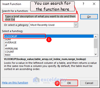
Solution 2: Use Insert Function Command

You can also use the Insert Function command to avoid errors like this.

• Select cell D14 and click on the Insert Function icon beside the Formula Bar.

It’ll open the Insert Function dialog box. In the Search for a function box, you can search for any function.

• Select the VLOOKUP function from the recently used functions and click OK. Otherwise, just double-click on the function to select it.

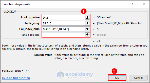
Instantly, the Function Arguments wizard pops up.

• In the respective boxes, give the arguments of the VLOOKUP function as we wrote in the formula. Here, you can select the range from the worksheet and it’ll be input as an argument automatically.
• Later, click OK.

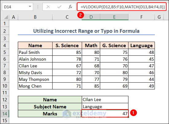
Witness the removal of the #NAME error, allowing the cell to exhibit the accurate output.

Reason 3: Causing #NAME Error If Named Range Is Not Defined

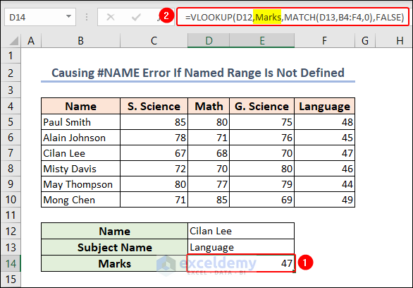
In the following formula, we used a named range (Marks) as the table_array argument of the VLOOKUP function.

But the formula returns the #NAME error in the output cell.

But, if we go back to the Dataset worksheet, and select the B4:F10 range, we can see the Marks named range in the Name Box. So, it means this named range is available in this workbook, so why doesn’t it work with the formula? Let’s search for the answer.

Solution: Make Use of Name Manager

Name Manager in Excel is a feature that allows you to view, create, edit, and delete named ranges and defined names in your workbook. It provides a central location to manage all the named ranges and names used in your formulas. To access it,

• Go to the Formulas tab >> Name Manager on the Defined Names group.

• In the Name Manager wizard, if you click on the Marks name, you can see the range of this name in the Refers to box. Actually, this named range is applicable to the Dataset worksheet only. That’s why it didn’t work in the formula of another sheet.
• Now, click on the New button at the top of this dialog box.

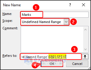
• In the New Name dialog box, fill up the following fields like the image below, and click OK.

Notice the absence of the #NAME error, resulting in the cell (D14) showing the correct output.

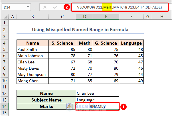
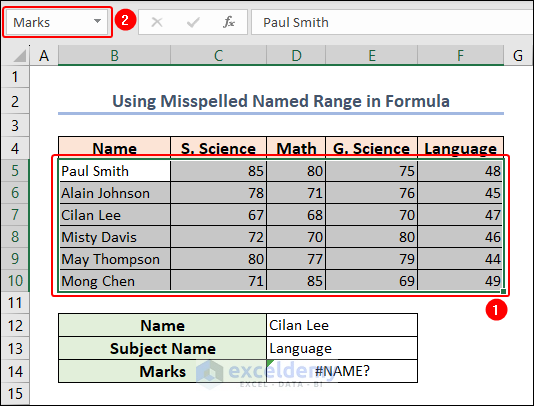
Reason 4: Using Misspelled Named Range in Formula

While you have so many named ranges for your dataset it is normal to forget the correct named range for using in a formula. We utilized the subsequent formula to carry out this task.

Here, Mark is a named range. But the formula isn’t working yet.

Solution: Select Range and Check the Name Box

You can use the Name Manager to solve this problem. Already, we showed it in the previous example.
Another way to resolve the issue is to select the range where we defined the range. Then, get a look into the Name Box at the left of the Formula bar. Here, you can find the right spelling of your named range.
In this case, it is Marks, but we wrote it as Mark in the formula. That’s why it returned an error.

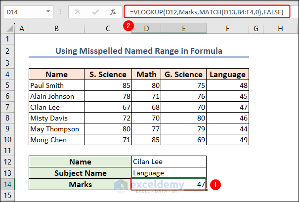
Now correct the range name in the formula and it looks like the following.

Observe how the #NAME error has vanished, leading to the cell presenting the correct result.

Reason 5: Writing Text String Without Quotation in Formula

If you write any text string in a formula without using a quotation sign for this string, then you will get the #NAME error instead of the correct result. Here, we used the text string Cilan Lee without any quotation in the following formula.

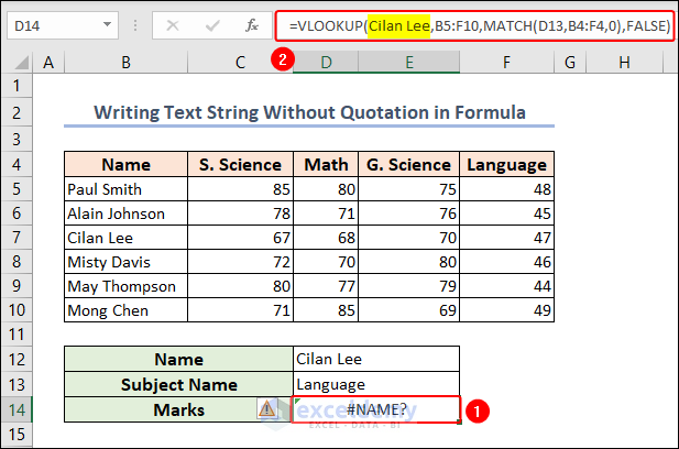
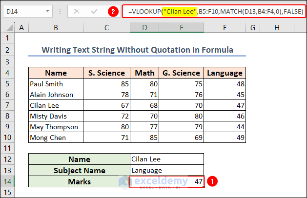
Solution: Use Double-Quote Around Text String

Just insert a pair of double quotes around the text string and the formula be like this:

Take note that Excel rectified the #NAME error, and the cell is now exhibiting the accurate output.

Reason 6: Returning #NAME Error for Compatibility Issue

The #NAME error occurs when there is a compatibility issue in Excel, leading to the inability to recognize a specific function or reference. This error is commonly encountered when using functions or features that are not supported in the current version of Excel.

For instance, dynamic array functions like UNIQUE, FILTER, SORT, and others, which were introduced in Excel 365, are unavailable in older versions. If any of these functions are attempted in Excel 2019 or earlier, a #NAME error will be generated.

Solution:

To address this issue, ensure that you are using a compatible version of Excel that supports the function or feature you are trying to use. Additionally, consider updating your Excel version or utilizing alternative methods or functions that are compatible with your current version.

By resolving the compatibility issue, you can eliminate the #NAME error and achieve the desired functionality in Excel.

Reason 7: Using Specific Functions Without Enabling Add-ins

If you come across the #NAME error, it could indicate that a specific formula requires an Add-in that is either not installed or enabled in your Excel.

For instance, when using the EUROCONVERT function, it necessitates enabling the Euro Currency Tools add-in. You can find it in the Excel Add-ins.

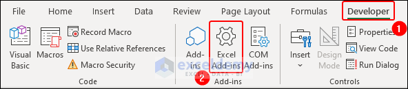
• In the Developer tab, click on Excel Add-ins in the Add-ins group.

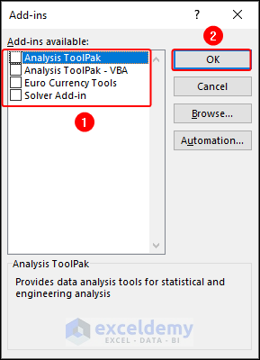
• In the Add-ins dialog box, select the necessary available add-in and click OK.

Moreover, Excel will return the same #NAME error, if you attempt to use any custom function which is not associated with the respective sheet.

How to Find #NAME Error in Excel

For a large dataset, it is difficult to find all of the #NAME errors properly. In this instance, you can see the following two methods.

1. Use Find and Replace Dialog Box

• First, go to Home >> Find & Select >> Find.

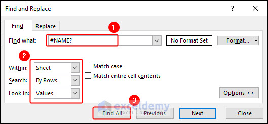
• In the Find and Replace dialog box, write the text string you want to find. Here, we want to locate the #NAME? error, so write this in the box.
• Then, select the following,

Within → Sheet
Search → By Rows
Look in → Values

• Next, click on Find All.

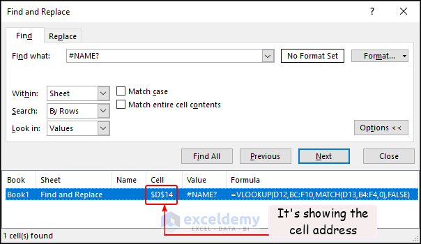
After that, you will get the cell address $D$14 which has the #NAME? error.

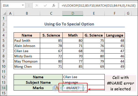
2. Use the Go To Special Option to Find #NAME Error

To use this option,

• Initially, navigate to Home >> Find & Select >> Go To Special.

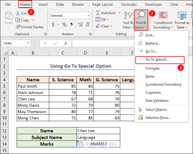
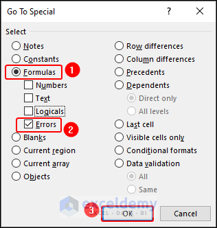
• In the Go To Special dialog box, check the radio button of Formulas and deselect all options except Errors inside it. Then, click OK.

Excel instantly selects the cell with the #NAME error. It can also select multiple cells with the same criteria.

Things to Remember

• Double-check the spelling and syntax of your formula. Even a small typo can result in a #NAME error.
• Keeping your Excel version up to date ensures that you have access to the latest functions and features.
• Implement proper error-handling techniques in your formulas to handle potential errors like #NAME. Use functions like IFERROR or ISERROR to handle errors gracefully and provide alternative outputs or error messages.
• If you are unable to resolve the #NAME? error using the above tips, consider seeking help from the Excel community. Excel Forum is a great platform in this case.

Frequently Asked Questions

1. What does the Name Error message look like in Excel?

The name error message is usually displayed as #NAME? in the cell where the error occurs. It indicates that Excel cannot recognize the name used in the formula or function.

2. Are there any built-in functions in Excel to help with Name Errors?

Yes, Excel provides some functions that can help handle name errors, such as ISERROR, ISNA, and IFERROR. These functions allow you to test for errors and provide alternative outputs or error-handling mechanisms in your formulas.

3. Can macros or VBA code contribute to Name Errors in Excel?

Yes, macros or VBA codes can potentially introduce name errors if they contain references to invalid or non-existent names.

4. Can circular references cause Name Errors?

Circular references can cause different types of errors in Excel, but they typically do not result in name errors. Circular references are more likely to cause Circular Reference or Ref# errors.

Download Practice Workbook

Download the following practice workbook. It will help you to realize the topic more clearly and will help you practice yourself.

Conclusion

In conclusion, name errors in Excel can be a common and frustrating issue that users may encounter while working with spreadsheets. These errors occur when a named range, function, or formula in Excel refers to a name that does not exist or is incorrectly defined.
Excel provides helpful error-checking features and formula auditing tools that can assist in identifying and resolving name errors. In this reference, we tried to demonstrate 7 different and valid reasons for this error. Also, we showed the corresponding solutions. Leveraging these, you can significantly simplify the troubleshooting process and enhance overall productivity.
Hope you will find it useful. If you have any suggestions or questions feel free to share them with us.

Related Articles

• On Error Resume Next: Handling Error in Excel VBA
• Excel VBA: Turn Off the “On Error Resume Next”
• [Fixed!] Error Messages in Excel
• [Fixed!] Error 509 in Excel
• How to Fix “Fixed Objects Will Move” in Excel