In this tutorial, you will learn how to make a Pie Chart in Excel without numbers. This type of situation is very common where you need people’s opinions on any issue. After collecting the opinions, you can generate a Pie Chart to visualize the data properly.
How to Make a Pie Chart in Excel without Numbers: 2 Effective Ways
1. Using Excel COUNTIF Function to Make Pie Chart without Numbers
The COUNTIF function in Excel counts the number of cells that meet a specified condition. This feature of the COUNTIF function is very helpful to make Pie Charts in Excel from data without numbers.
1.1 For Yes/No Answer
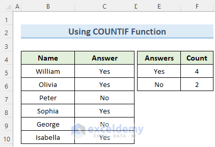
For this method, we have a dataset that contains the answers people gave on whether they were infected with Covid–19. Obviously, all the answers are only either Yes or No. Let us see how we can use this data to create a Pie Chart.
Steps:
- First of all, select cell F5 and type in the following formula:
- Then, press Enter.
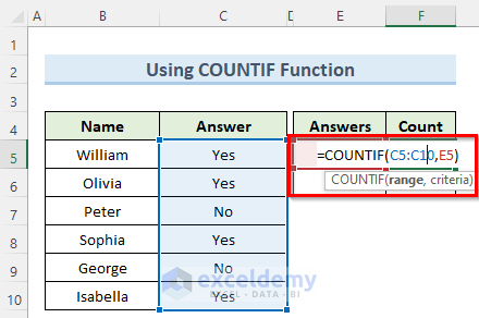
- As a result, the formula will count the number of times the option Yes is found in the data table.
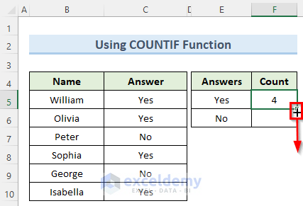
- Now, click and drag the Fill handle tool to copy the formula to the cell below.
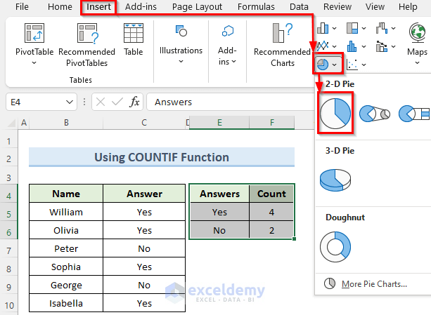
- After that, select the table from cell E4 to F6 and navigate to the Insert tab.
- Below the Insert tab, click the Insert Pie Chart drop-down.
- From there, click on the 2-D Pie option.
- Thus, you will get a nice and clear Pie Chart representing your data.

1.2 For Multiple Answers
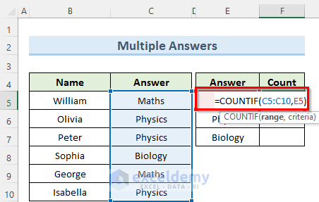
In this method, we have the dataset of students’ answers on their favorite subject. Unlike the first method, here we have multiple answers to the question. This type of dataset is very common in real-life situations. So, follow the steps below to get a Pie Chart from this data.
Steps:
- To begin with, select cell F5 and enter the following formula:
- Note that, you can also type the formula directly into the formula bar.
- Now, press Enter and copy the formula to the cells below using the Fill Handle.
- Then, select the table from cell E4 to F7 and go to the Insert tab above.
- There, click on the Insert Pie Chart drop-down and select 2-D Pie.
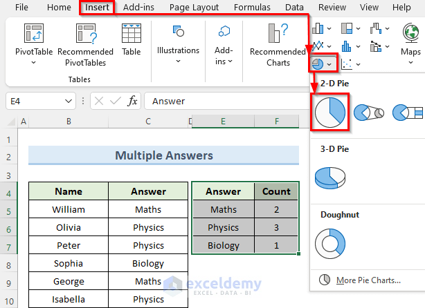
- As a result, Excel will generate a Pie Chart showing the proportions of the answers.

Read More: How to Make a Pie Chart with Multiple Data in Excel
2. Make Pie Chart in Excel Using Pivot Chart
We can easily create a Pie Chart for data without numbers using Pivot Charts. We are using the same data set from the first method to keep things simple. Let us jump right into this final method.
Steps:
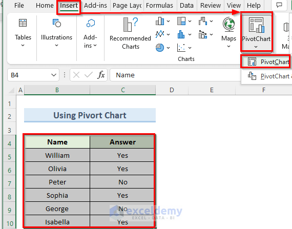
- First, select the dataset from cells B4 to C10.
- Second, go to the Insert tab and select the PivotChart dropdown.
- Below this, click on the PivotChart option.
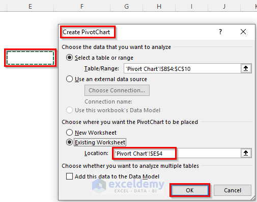
- Now, in the new Create PivotChart window, select the option Existing Worksheet.
- After that, click on an empty cell in column E and press OK.
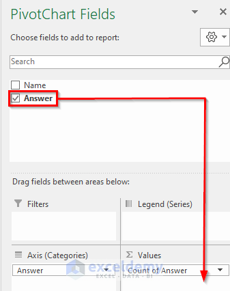
- Then, on the right, a new PivotChart Fields window opens.
- Here, check the Answer option and drag the Answer option to the Values section.
- Now, you will see a pivot chart on the worksheet.
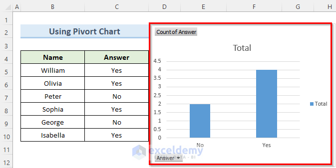
- Next, right-click on any of the bars on the pivot chart.
- Then, from the options menu select Change Series Chart Type.

- After that, in the Change Chart Type window select Pie and press OK.
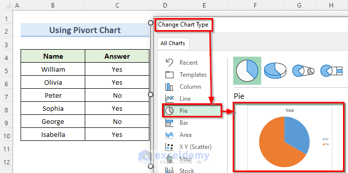
- Finally, the last operation will convert the pivot chart into a Pie Chart.

Read More: How to Create a Pie Chart in Excel from Pivot Table
Conclusion
I hope that you thoroughly understood the methods I showed in this tutorial to make a Pie Chart in Excel without numbers. You should keep in mind that, you can only create Pie Charts for a single column or row of data. Also, Pie Charts are not very suitable for many data cells. With that said, I would encourage you to try some formatting on your Pie Chart and make it more readable. And lastly, to learn more Excel techniques, follow our ExcelDemy website. If you have any queries, please let me know in the comments.
Related Articles
- How to Make Pie Chart in Excel with Subcategories
- How to Make Pie Chart with Breakout in Excel
- How to Make Two Pie Charts with One Legend in Excel
- How to Make a Pie Chart in Excel with One Column of Data
- How to Make a Pie Chart in Excel with Words
<< Go Back To Make a Pie Chart in Excel | Excel Pie Chart | Excel Charts | Learn Excel
Get FREE Advanced Excel Exercises with Solutions!
