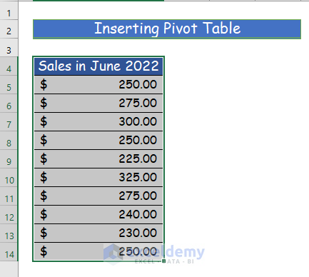
This is the sample dataset.

Method 1 – Inserting a PivotTable to Create a Pie Chart in Excel
Step 1:
- Select the entire column. Here, B4:B14.
Step 2:
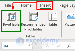
- Go to the Insert tab and choose PivotTable.
Step 3:
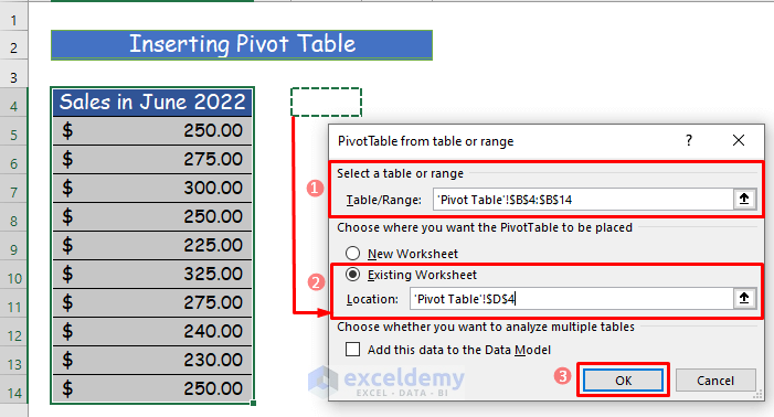
- In “Select a table or range”, you will see the selected range (B4:B14).
- Select “Existing Worksheet” and choose an empty cell near your dataset. Here, D4.
- Click OK.
Step 4:
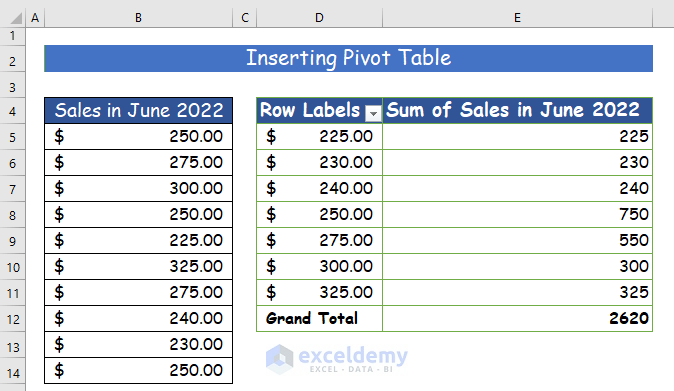
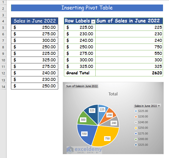
- In “PivotTable Fields”, drag Sales in June 2022 to both Rows and Values.
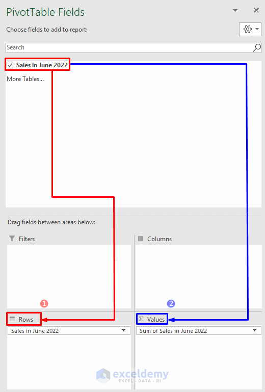
The PivotTable is displayed.
Step 5:
- Select any cell in the table.
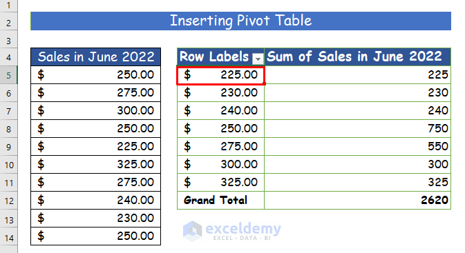
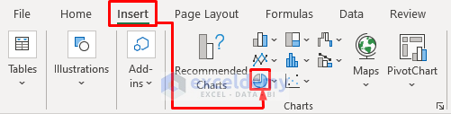
Step 6:
- Go to the Insert tab and click “Insert Pie or Doughnut Chart” in Charts.
Step 7:
- Choose a pie model. Here, 2-D Pie.
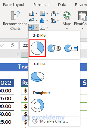
The pie chart is displayed.
Read More: How to Create a Pie Chart in Excel from Pivot Table
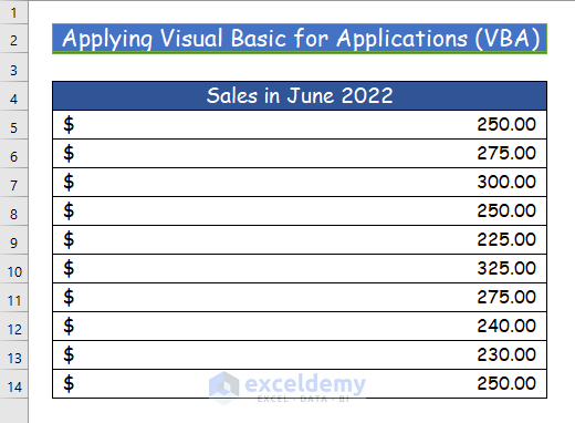
Method 2 – Applying VBA to Create a Pie Chart in Excel
Step 1:
- Use the following dataset:
Step 2:
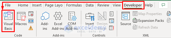
- Go to the Developer tab and choose Visual Basic.
Step 3:
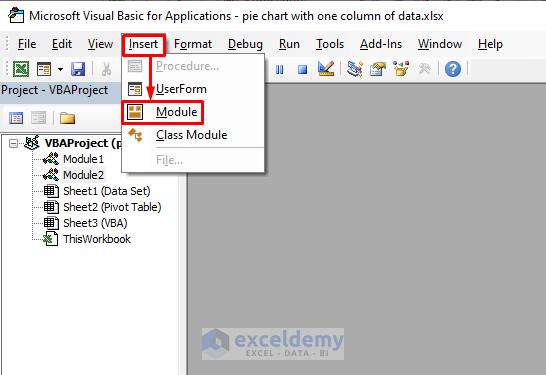
- In the Insert tab, choose Module.
Step 4:
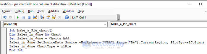
- Enter the following VBA Code.
Sub Make_a_Pie_chart()
Dim Sales_in_June As Chart
Set Sales_in_June = Charts.Add
Sales_in_June.SetSourceData Source:=Worksheets("VBA").Range("B4").CurrentRegion, PlotBy:=xlColumns
Sales_in_June.ChartType = xlPie
End Sub
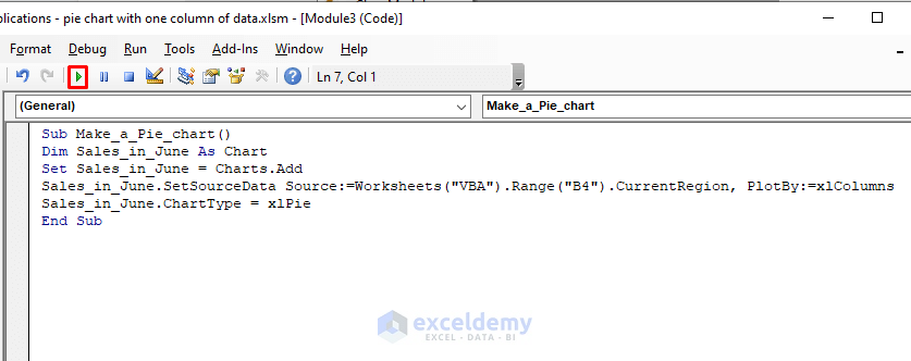
Step 5:
- Save the program and press the play button to run the code.
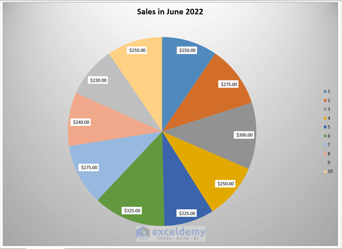
You will see the pie chart:
Read More: How to Make a Pie Chart with Multiple Data in Excel
Download Practice Workbook
Related Articles
- How to Make Pie Chart in Excel with Subcategories
- How to Make a Pie Chart in Excel with Words
- How to Make a Pie Chart in Excel without Numbers
<< Go Back To Make a Pie Chart in Excel | Excel Pie Chart | Excel Charts | Learn Excel
Get FREE Advanced Excel Exercises with Solutions!
