How to Create a Budget Pie Chart in Excel – 7 Easy Steps

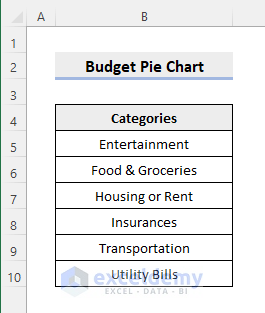
Step 1- Set Budget Categories

• Enter the budget categories in B5:B10, here.

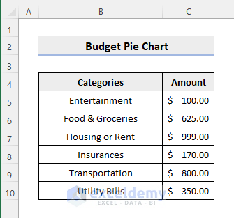
Step 2 -Enter Budget Amounts

• Enter the expenses in C5:C10.

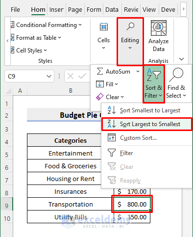
Step 3 – Format the Budget Table

• Select any cell in the dataset containing the amounts.
• Go to the Home tab.
• Select Sort & Filter in Editing.
• Click Largest to Smallest or Smallest to Largest to sort data.

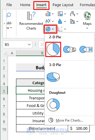
Step 4 – Insert the Pie Chart

• Select a cell in the dataset.
• In Insert, select Charts.
• Click Insert Pie or Doughnut Chart.
• Choose 2-D Pie.

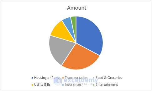
This is the output.

Read More: How to Make a Pie Chart in Excel

Step 5 – Edit the Budget Pie Chart

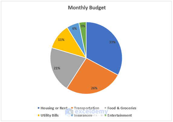
• Click the chart title (Amount) and rename it (Monthly Budget).

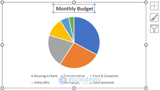
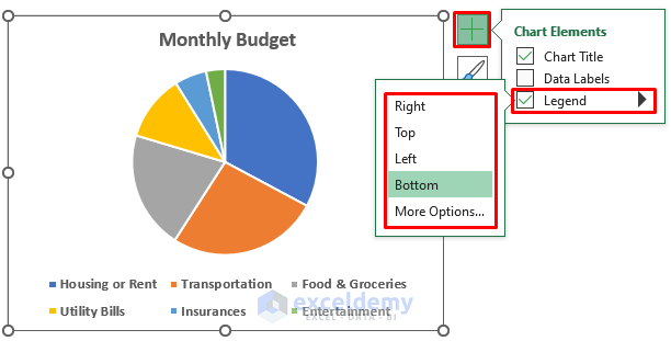
• Click Chart Elements (+) at the upper-right corner.

You can show/hide the categories using the Legend.

• Click Right to show the categories on the right side of the chart

You can also click the categories to bold or increase the font size.

• Check Data Labels to show the amounts on the chart. If you want to show the percentage only, select More Options.

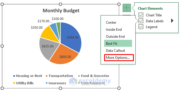
• In Format Data Labels, check Percentage and uncheck Value.

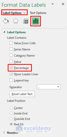
Only the percentages will be displayed.

Read More: How to Make Multiple Pie Charts from One Table

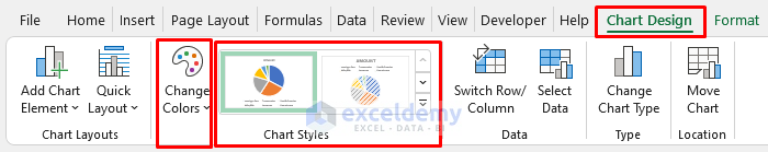
Step 6 -Format the Budget Pie Chart

• Click the chart to access the Chart Design tab or format it in the Format tab.

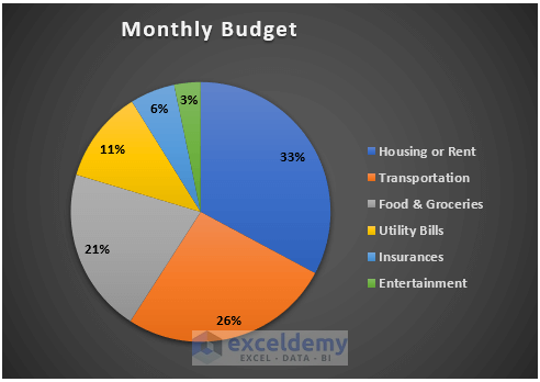
Step 7 – Finalize the Budget Pie Chart

This is the output.

Read More: How to Create a 3D Pie Chart in Excel

Download Practice Workbook

Related Articles

• How to Make a Gender Pie Chart in Excel
• How to Make Pie of Pie Chart in Excel
• How to Create & Customize Bar of Pie Chart in Excel
• How to Make a Multi-Level Pie Chart in Excel

<< Go Back To Make a Pie Chart in Excel | Excel Pie Chart | Excel Charts | Learn Excel