How to Make Multiple Pie Charts from One Table (3 Easy Ways)

Looking for ways to know how to make multiple pie charts from one table in Excel? We can make multiple pie charts from one table by going through some easy steps. Here, you will find step-by-step explained ways to make multiple pie charts from one table in Excel.

How to Make Multiple Pie Charts from One Table: 3 Ways

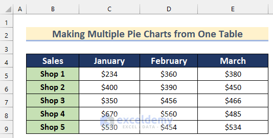
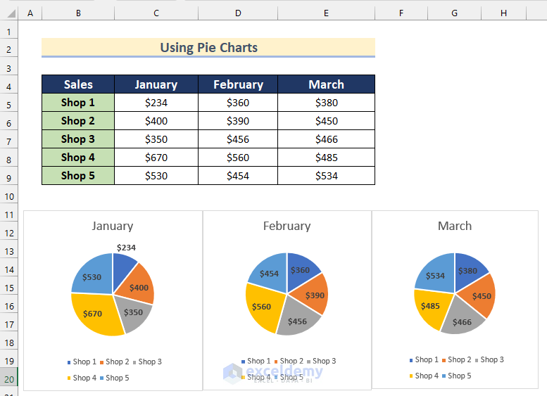
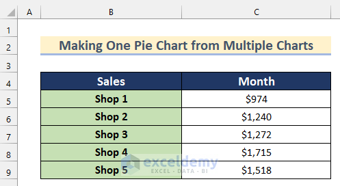
Here, we have a dataset containing the data of Sales for consecutive 3 months January, February, and March of 5 Shops. Now, we will use this dataset to show you how to make multiple Pie Charts from one table in Excel.

1. Using Pie Charts Feature in Excel

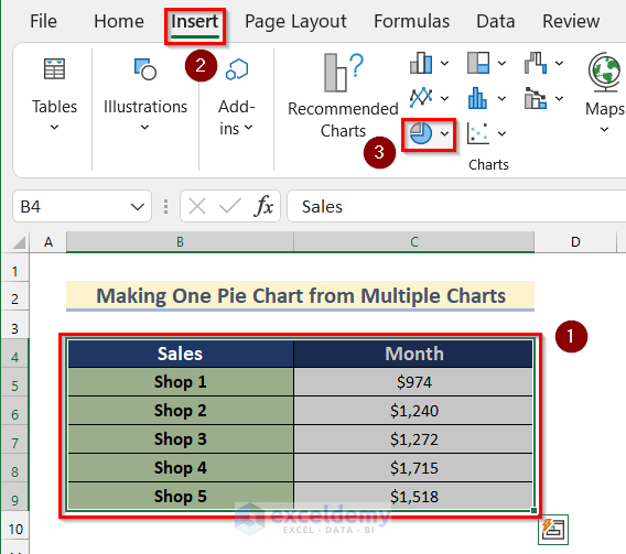
In the first method, we will use Pie Charts to make pie charts from one table. Go through the steps to do it on your dataset.

Steps:

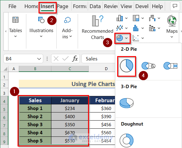
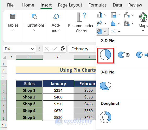
In the beginning, select Cell range B4:C9.
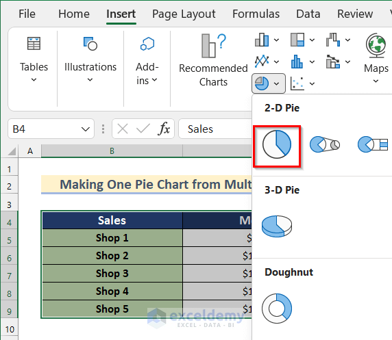
Then, go to the Insert tab >> click on Pie Chart >> select 2-D Pie chart.

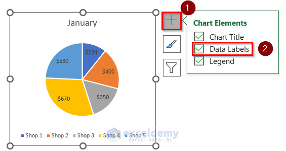
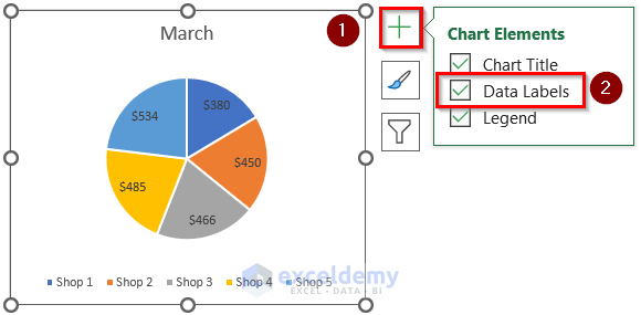
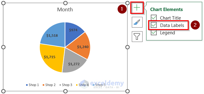
Now, a Pie Chart will appear containing the Sales data of January.
After that, click on the “+” sign to open Chart Elements.
Next, turn on Data Labels.

Then, select Cell range B4:B9 and D4:D9.
Afterward, go to the Insert tab >> click on Pie Chart.

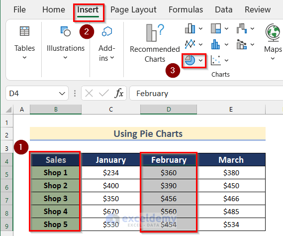
Next, select the 2-D Pie chart.

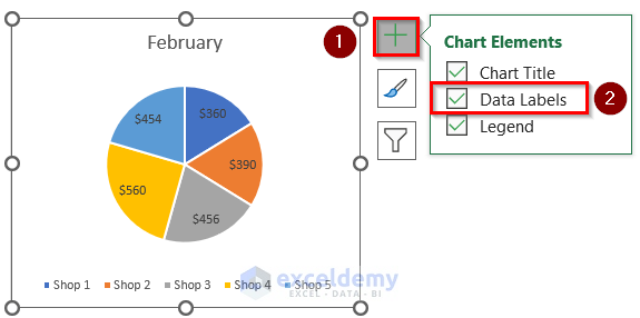
Now, a Pie Chart will appear containing the Sales data of February.
After that, click on the “+” sign to open Chart Elements.
Then, turn on Data Labels.

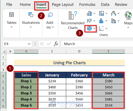
Next, select Cell range B4:B9 and E4:E9.
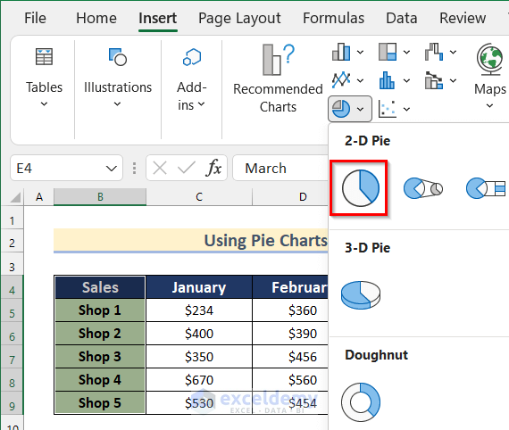
After that, go to the Insert tab >> click on Pie Chart.

Then, select the 2-D Pie chart.

Now, a Pie Chart will appear containing the Sales data of March.
Afterward, click on the “+” sign to open Chart Elements.
Next, turn on Data Labels.

Finally, you will get 3 separate Pie Charts for January, February and March from one table using Pie Charts.

Read More: How to Make a Pie Chart in Excel

2. Applying Doughnut Chart to Make Two Pie Charts in One from One Table

Now, we will show you how to apply a Doughnut Chart to make two Pie Charts in one from one table in Excel.

Follow the steps given below to do this on your own.

Steps:

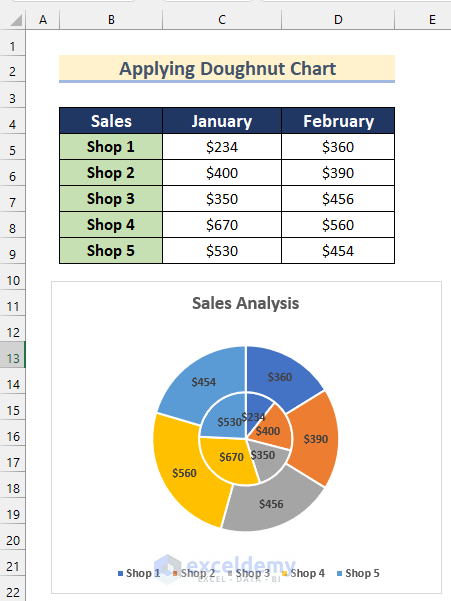
First, select Cell range B4:D9.
Then, go to the Insert tab >> click on Pie Chart.

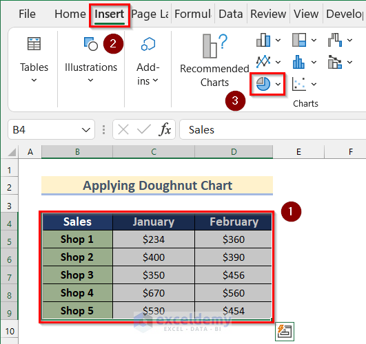
After that, select the Doughnut chart.

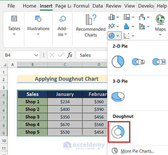
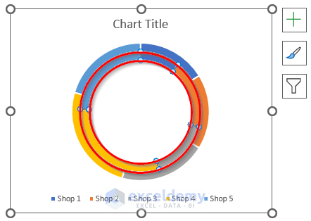
Now, a Doughnut chart will appear containing the Sales data of January and February.
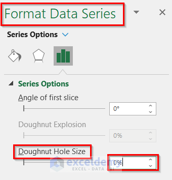
Next, select the smaller Doughnut chart.

Then, the Format Data Series toolbox will open.
Afterward, insert 0% in the Doughnut Hole Size box.

Next, click on the Chart Title to change it.

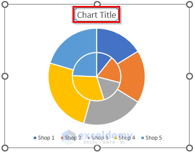
Now, type Sales Analysis as Chart Title.

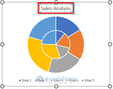
After that, click on the “+” sign to open Chart Elements.
Then, turn on Data Labels.

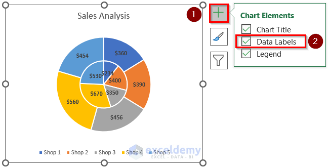
Finally, you will get two Pie Charts in one from one table by applying the Doughnut Chart.

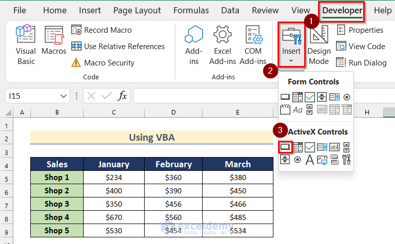
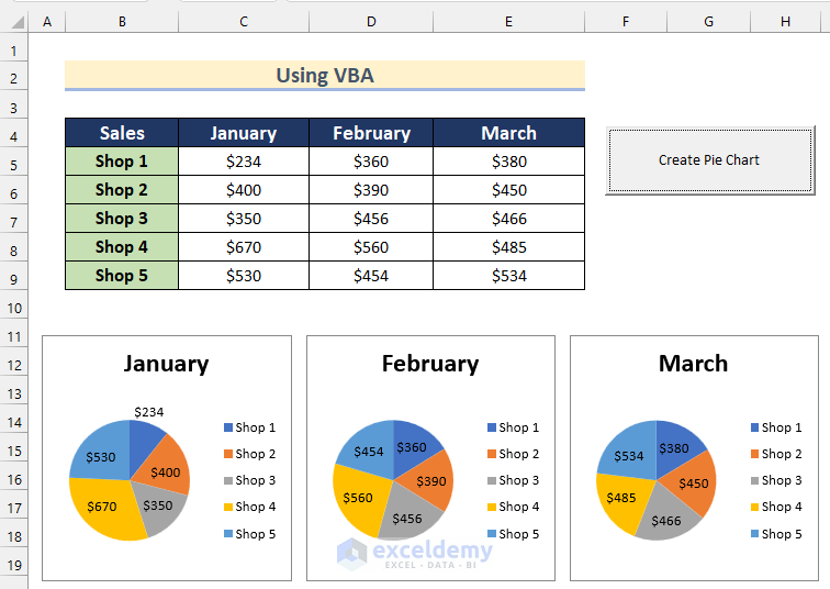
3. Using VBA to Make Multiple Pie Charts from One Table

In the final method, we will use VBA to make multiple pie charts from one table. Go through the steps to do it on your own.

Steps:

In the beginning, go to the Developer tab >> click on Insert >> select Command Button.

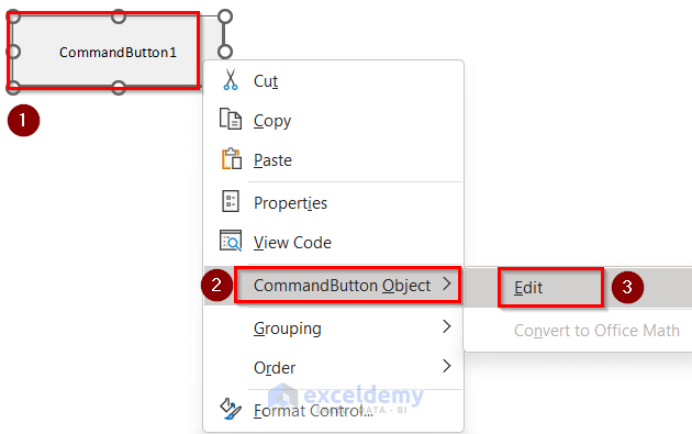
Then, insert CommandButton1.
After that, Right-click on the button.
Next, click on CommandButton Object >> select Edit.

Now, type Create Pie Chart to edit the Command Button.

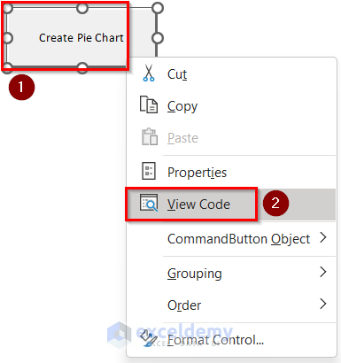
Then, Right-click on the Create Pie Chart button.
Next, select View Code.

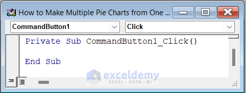
Now, you will see the code for CommandButton1_Click.

Next, write the following code in your Module.

Option Explicit
Private Sub CommandButton1_Click()
    Multiple_Pie_Charts
End Sub
Sub Multiple_Pie_Charts()
    Dim Sales As Worksheet
    Set Sales = Worksheets("Using VBA")
    Dim sales_chart As ChartObject
    For Each sales_chart In Sales.ChartObjects
        sales_chart.Delete
    Next
    Dim Rng() As String
    ReDim Rng(1 To 4)
    Rng(1) = "C5"
    Rng(2) = "D5"
    Rng(3) = "E5"
    Dim Sales_Pie_Chart As New Chart
    Dim Sells_Series As Series
    Dim row_number As Integer
    Dim move_left  As Integer
    move_left = 10
    For row_number = LBound(Rng) To UBound(Rng) - 1
        Set Sales_Pie_Chart = Sales.ChartObjects.Add _
        (Width:=170, Height:=170, _
            Top:=210, Left:=move_left).Chart
        With Sales_Pie_Chart
            .ChartType = xlPie
            .HasTitle = True
            .ChartTitle.Text = Sales.UsedRange.Rows.Cells _
            (3, row_number + 1)
            Set Sells_Series = .SeriesCollection.NewSeries
            With Sells_Series
                .XValues = Sales.Range(Sales.Range("B5"), _
                Sales.Range("B5").End(xlDown))
                .Values = Sales.Range(Sales.Range(Rng(row_number)), _
                Sales.Range(Rng(row_number)).End(xlDown))
            End With
            .SeriesCollection(1).HasDataLabels = True
        End With
        move_left = move_left + 180
    Next row_number
End Sub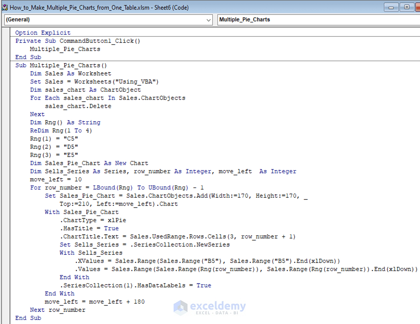

Code Breakdown

First, we created Sub Procedure as Multiple_Pie_Charts().
Then, we declared Sales as Worksheet.
After that, we set the Sales from Using VBA Worksheet.
Next, we declared sales_chart as ChartObject.
Then, we created a For loop for each sales_chart in the Sales worksheet to delete previous charts while creating new charts.
Afterward, we declared Rng() as String and redeclared Rng from 1 to 4.
Next, we inserted Rng(1) =”C5″ ,Rng(2) =”D5″ and Rng(3) =”E5″.
Then, we declared Sales_Pie_Chart as a New Chart, Sells_Series as Series, row_number as Integer and move_left as Integer.
After that, we inserted move_left=10.
Again, we used a For loop for row_number Lower Bound of Rng to Upper Bound of Rng subtracted by 1.
Next, we set the Sales_Pie_Chart as a Chart containing Width=170, Height= 170, Top=210 and Left=move_left.
Then, with the Sales_Pie_Chart we selected xlPie as ChartType, set Title as True and set the value as Cell (3, row_number+1) where values of the given row & column will be displayed as Chart Title.
After that, with Sells_series we inserted XValues from the Sales worksheet as Cell B5.
Moreover, we inserted Values from the Sales worksheet as Rng(row_number).
Then, we set the Data Labels as True.
After that, we inserted move_left= move_left+180 it will shift the Charts towards right and will create a gap between charts.

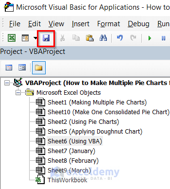
Next, click on the Save button and go back to your worksheet.

After that, click on the Create Pie Chart button.
Finally, you will get 3 separate Pie Charts for January, February and March from one table using VBA.

Make One Pie Chart from Multiple Tables

We can also make one pie chart from multiple tables in Excel by going through some steps.

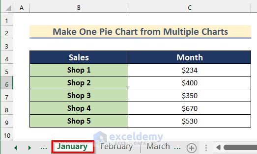
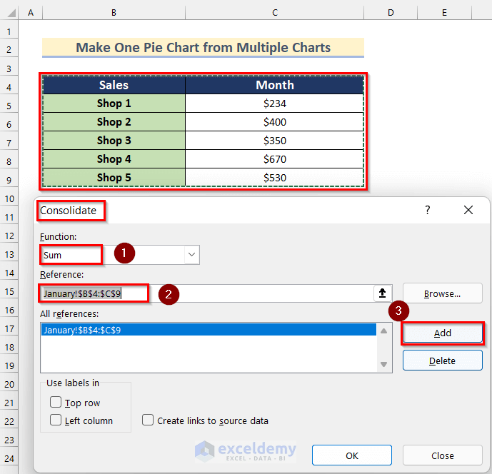
Here, the above data set shows the values of Sales of the Shops in January.

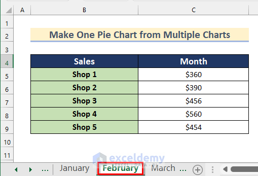
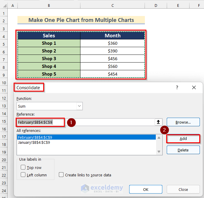
The above data set shows the values of Sales of the Shops in February.

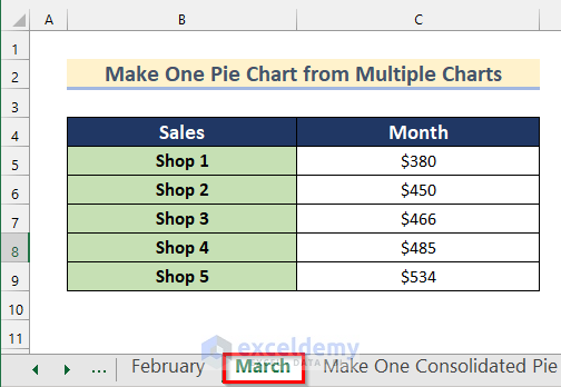
Finally, the above data set shows the values of Sales of the Shops in March.

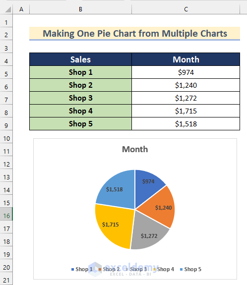
Now, we will consolidate the Sales value of the 3 months using the Consolidate Feature. Follow the steps below to do it on your own.

Steps:

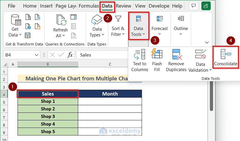
First, open a new Worksheet and prepare the worksheet for the consolidated data.

Then, select Cell B4.
After that, go to the Data tab >> click on Data Tools >> select Consolidate.

Then, the Consolidate dialog box will open.
Now, select Sum as Function.
Next, in the Reference box insert the Cell range B4:C9 from the worksheet January.
After that, press Add.

Again, in the Reference box insert the Cell range B4:C9 from the worksheet February.
Then, press Add.

Now, in the Reference box insert the Cell range B4:C14 from the worksheet February.
After that, press Add.

Next, activate the Top row and Left column.
Then, press OK.

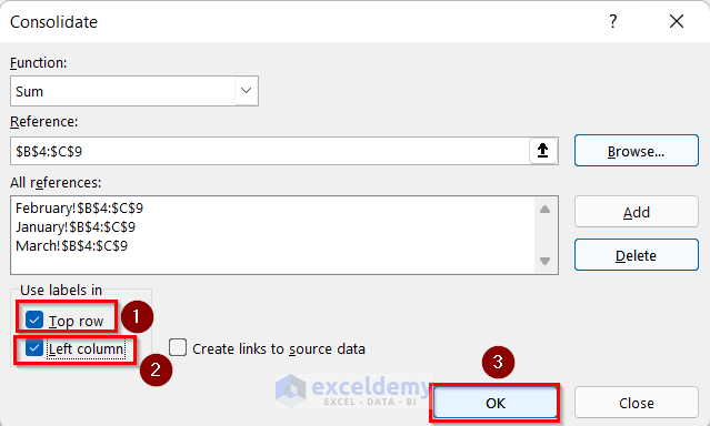
Finally, you will find the consolidated sum of Sales values of the three consecutive months applying the Consolidate Feature.

Afterward, go to the Insert tab >> click on Pie Charts.

Then, select the 2-D Pie chart.

After that, click on the “+” sign to open Chart Elements.
Next, turn on Data Labels.

Finally, you will get one pie chart from multiple tables in Excel.

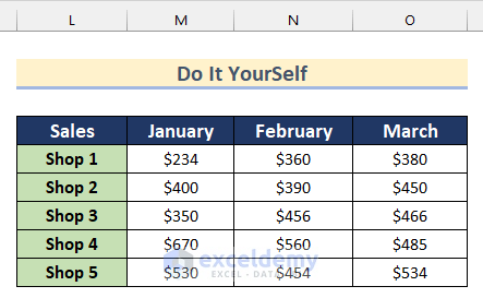
Practice Section

In this section, we are giving you the dataset to practice on your own and learn to use these methods.

Download Practice Workbook

Making Multiple Pie Charts.xlsm

Conclusion

So, in this article, you will find a step-by-step way to make multiple pie charts from one table in Excel. Use any of these ways to accomplish the result in this regard. Hope you find this article helpful and informative. Feel free to comment if something seems difficult to understand. Let us know any other approaches which we might have missed here. And, visit ExcelDemy for many more articles like this. Thank you!

<< Go Back To Make a Pie Chart in Excel | Excel Pie Chart | Excel Charts | Learn Excel

Get FREE Advanced Excel Exercises with Solutions!

How to Make Multiple Pie Charts from One Table (3 Easy Ways)

How to Make Multiple Pie Charts from One Table: 3 Ways

1. Using Pie Charts Feature in Excel

2. Applying Doughnut Chart to Make Two Pie Charts in One from One Table

3. Using VBA to Make Multiple Pie Charts from One Table

Make One Pie Chart from Multiple Tables

Practice Section

Conclusion

Related Articles

Leave a reply Cancel reply