What is a Pie Chart?
A Pie Chart is a circular graph where each slice represents a proportionate part of the entire dataset. In Microsoft Excel, creating a chart from a PivotTable is referred to as a PivotChart, although it functions similarly to a regular chart.
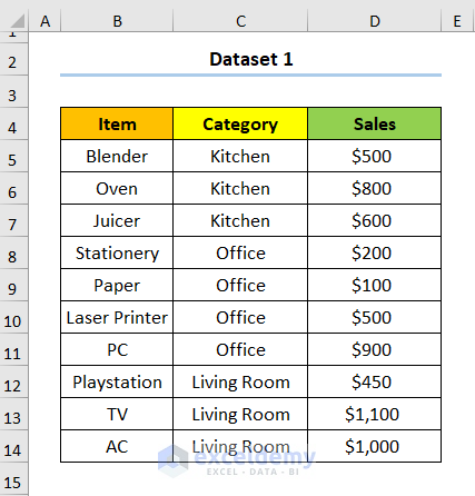
Dataset Overview
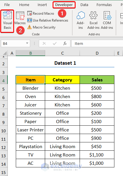
Let’s work with the following dataset located in cells B4:D14:
- Column B: Item names
- Column C: Categories
- Column D: Sales (in USD)
Method 1 – Creating a Pie Chart from Pivot Table in Excel
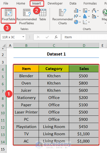
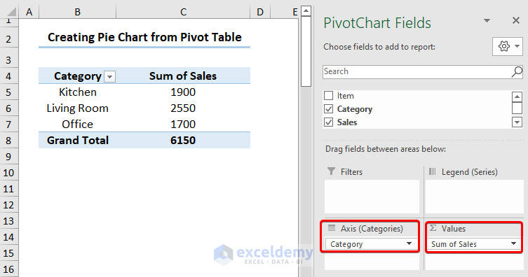
Step 1 – Insert a Pivot Table
- Select the dataset and go to Insert and click on PivotTable.
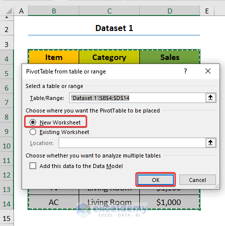
- In the dialog box, check the New Worksheet option and click OK.
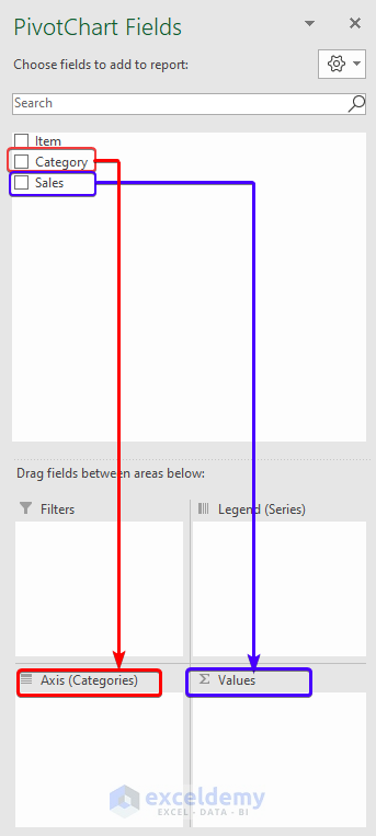
- Drag the Category field to the Axis (Categories) area and the Sales field to the Values area.
- A table will be generated automatically.
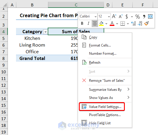
Step 2 – Format Numeric Values
- Right-click on the numeric values and select Field Value Settings.
- Click the Number Format button.
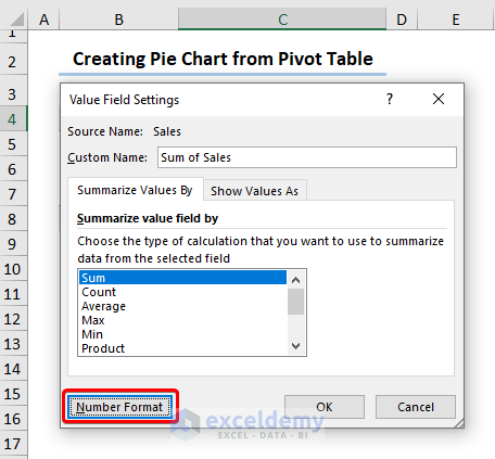
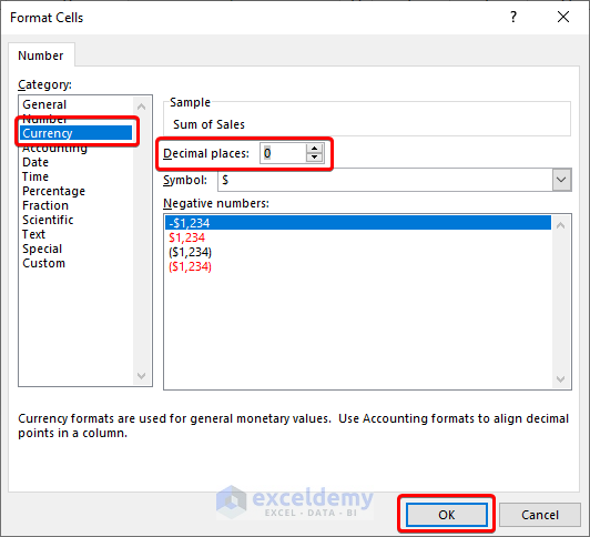
- Choose the Currency option (we chose 0 decimal places for Sales).
Step 3 – Create the Pie Chart
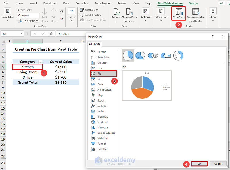
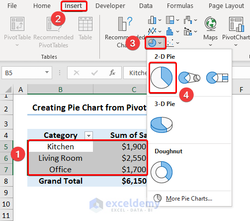
- Select any cell in the PivotTable.
- Go to PivotChart, select Pie (or use Insert, select Insert Pie or Doughnut Chart and click on Pie).
- Customize the chart by clicking on Chart Elements.
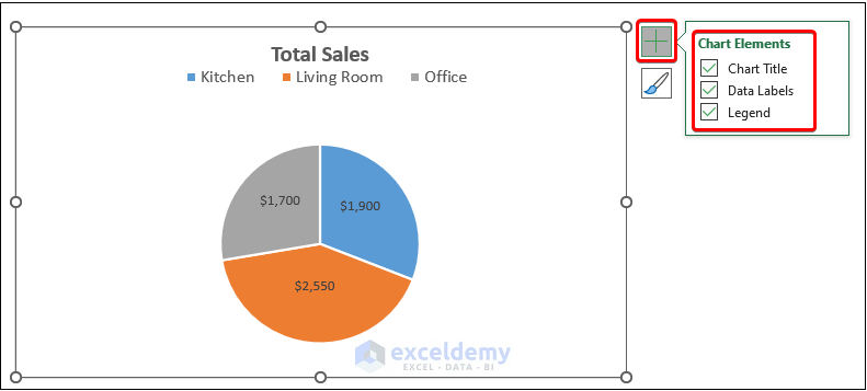
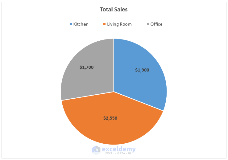
The results should look like the screenshot below:
Read More: How to Make Pie Chart in Excel with Subcategories
Method 2 – Using VBA to Insert a Pie Chart from a Pivot Table
If you frequently create Pie Charts from PivotTables, consider using the following VBA code:
Step 1 – Open the Visual Basic Editor
- Go to Developer and select Visual Basic.
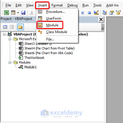
Step 2 – Insert the VBA Code
- Navigate to Insert, choose Module and paste the following code:
Option Explicit
Sub CreatePivotTable()
Dim pt As PivotTable
Dim pc As PivotCache
Sheet3.Activate
Set pc = ActiveWorkbook.PivotCaches.Create(xlDatabase, Range("B4").CurrentRegion)
Sheets.Add , Sheets(Sheets.Count)
Set pt = ActiveSheet.PivotTables.Add(pc, Range("B4"), "Sales_Pivot")
pt.PivotFields("Category").Orientation = xlRowField
pt.PivotFields("Sales").Orientation = xlDataField
End Sub
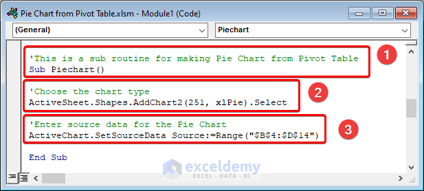
Sub Piechart()
ActiveSheet.Shapes.AddChart2(251, xlPie).Select
ActiveChart.SetSourceData Source:=Range("$B$4:$D$14")
End Sub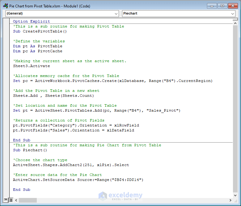
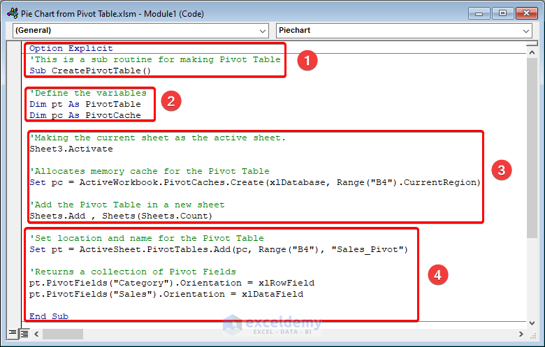
Code Breakdown
The code is divided into two sections:
Section 1 – Explanation of CreatePivotTable () sub-routine
- 1- Assign a name for the sub-routine.
- 2- Define the variables.
- 3- Sheet3 is activated using the Activate method and the memory cache is assigned using the PivotCache object.
- Additionally, we insert the PivotTable in a new sheet with the Add method.
- 4- Position the PivotTable in the B4 cell and give the name Sales_Pivot.
- We add the Pivot Fields i.e. the Category in the RowField and Sales in the DataField.
Section 2 – Description of Piechart () sub-routine
- 1- In this section, give a name to the sub-routine.
- 2- The ActiveSheet property inserts the Pie Chart using the Shapes.AddChart2 method.
- 3- The SourceData property selects the data range for the Pie Chart.
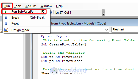
Step 3 – Run the VBA Code
- Press F5 to run the CreatePivotTable() sub-routine.
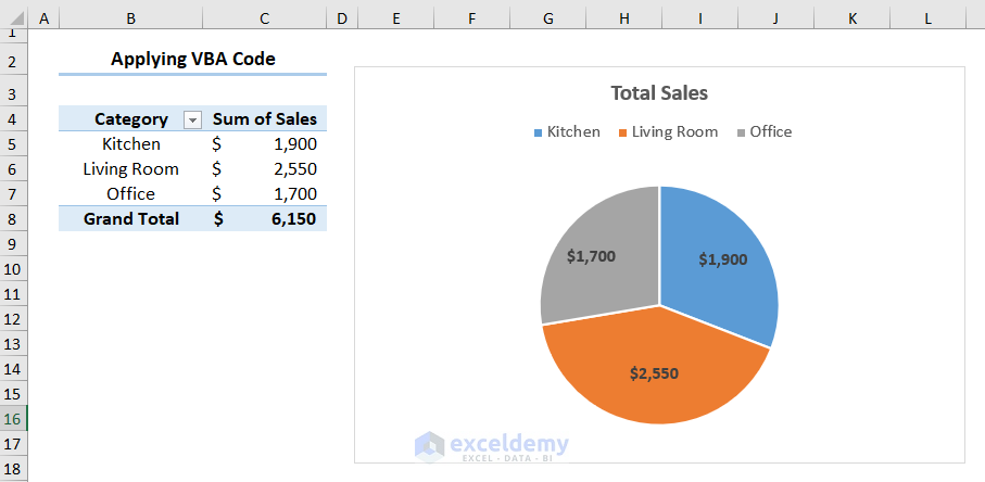
- Execute the Piechart() sub-routine.
- The result should resemble the screenshot below.
Read More: How to Make a Pie Chart with Multiple Data in Excel
Download Practice Workbook
You can download the practice workbook from here:
Related Articles
- How to Make a Pie Chart in Excel with One Column of Data
- How to Make a Pie Chart in Excel with Words
- How to Make a Pie Chart in Excel without Numbers
<< Go Back To Make a Pie Chart in Excel | Excel Pie Chart | Excel Charts | Learn Excel
Get FREE Advanced Excel Exercises with Solutions!
